Using Undefined or Defined Variables
When performing algebraic or calculus operations, it is important that you understand the effect of using undefined and defined variables. Otherwise, you may get a number for a result instead of the algebraic expression that you anticipated.
How Undefined and Defined Variables Are Treated
When you enter an expression that contains a variable, the TI-89 / TI-92 Plus treats the variable in one of two ways.
-
If the variable is undefined, it is treated as an algebraic symbol.
-
If the variable is defined (even if defined as 0), its value replaces the variable.
Tip: When defining a variable, it's a good practice to use more than one character in the name. Leave one-character names undefined for symbolic calculations.
To see why this is important, suppose you want to find the first derivative of $x^3$ with respect to x.
-
If x is undefined, the result is in the form you probably expected.
-
If x is defined, the result may be in a form you did not expect.
Unless you knew that 5 had been stored to x previously, the answer 75 could be misleading.
Determining If a Variable Is Undefined
Method: Example:
Enter the variable name. If defined, the variable's value is displayed.
If undefined, the variable name is displayed.
Use the getType function. If defined, the variable's type is displayed.
If undefined, "NONE" is displayed.
Note: Use [2nd] [VAR-LINK] to view a list of defined variables, as described in Chapter 21.
Chapter 3: Symbolic Manipulation 59


Deleting a Defined Variable
You can “undefine” a defined variable by deleting it.
| To delete: | Do this: |
|---|---|
| One or more specified variables | Use the DelVar function. |

You can also delete variables by using the VAR-LINK screen ([2nd] [VAR-LINK]) as described in Chapter 21.
Note: For information about folders, refer to Chapter 5.
| All one-letter variables (a – z) in the current folder | From the Home screen Clean Up menu, select 1:Clear a-z. You will be prompted to press [ENTER] to confirm the deletion. |
|---|---|
Temporarily Overriding a Variable
By using the “with” operator (|), you can:
-
Temporarily override a variable’s defined value.
-
Temporarily define a value for an undefined variable.
Note: For more information about the | operator, refer to page 67.
To type the “with” operator (|), press:
TI-89: [ | ]
TI-92 Plus: [2nd] [ | ]
60 Chapter 3: Symbolic Manipulation
Using Exact, Approximate, and Auto Modes
The Exact/Approx mode settings, which are described briefly in Chapter 2, directly affect the precision and accuracy with which the TI-89 / TI-92 Plus calculates a result. This section describes these mode settings as they relate to symbolic manipulation.
EXACT Setting
When Exact/Approx = EXACT, the TI-89 / TI-92 Plus uses exact rational arithmetic with up to 614 digits in the numerator and 614 digits in the denominator. The EXACT setting:
- Transforms irrational numbers to standard forms as much as possible without approximating them. For example, \sqrt12 transforms to 2\sqrt3 and \ln(1000) transforms to 3\ln(10).
- Converts floating-point numbers to rational numbers. For example, 0.25 transforms to 1/4.
The functions solve, cSolve, zeros, cZeros, factor, ∫, fMin, and fMax use only exact symbolic algorithms. These functions do not compute approximate solutions in the EXACT setting.
- Some equations, such as $2^{-x} = x$, have solutions that cannot all be finitely represented in terms of the functions and operators on the TI-89 / TI-92 Plus.
- With this kind of equation, EXACT will not compute approximate solutions. For example, $2^{-x} = x$ has an approximate solution x \approx 0.641186, but it is not displayed in the EXACT setting.
| Advantages | Disadvantages |
|---|---|
| Results are exact. | As you use more complicated rational numbers and irrational constants, calculations can: |
| - Use more memory, which may exhaust the memory before a solution is completed. | |
| - Take more computing time. | |
| - Produce bulky results that are harder to comprehend than a floating-point number. |
Chapter 3: Symbolic Manipulation 61
APPROXIMATE Setting
When Exact/Approx = APPROXIMATE, the TI-89 / TI-92 Plus converts rational numbers and irrational constants to floating-point. However, there are exceptions:
- Certain built-in functions that expect one of their arguments to be an integer will convert that number to an integer if possible. For example:
d(y(x), x, 2.0)transforms tod(y(x), x, 2). - Whole-number floating-point exponents are converted to integers. For example: x².⁰ transforms to x² even in the APPROXIMATE setting.
Functions such as solve and ∫ (integrate) can use both exact symbolic and approximate numeric techniques. These functions skip all or some of their exact symbolic techniques in the APPROXIMATE setting.
| Advantages | Disadvantages |
|---|---|
| If exact results are not needed, this might save time and/or use less memory than the EXACT setting. | Results with undefined variables or functions often exhibit incomplete cancellation. For example, a coefficient that should be 0 might be displayed as a small magnitude such as 1.23457E-11. |
| Approximate results are sometimes more compact and comprehensible than exact results. | Symbolic operations such as limits and integration are less likely to give satisfying results in the APPROXIMATE setting. |
| If you do not plan to use symbolic computations, approximate results are similar to familiar, traditional numeric calculators. | Approximate results are sometimes less compact and comprehensible than exact results. For example, you may prefer to see 1/7 instead of .142857. |
62 Chapter 3: Symbolic Manipulation
AUTO Setting
When Exact/Approx = AUTO, the TI-89 / TI-92 Plus uses exact rational arithmetic wherever all of the operands are rational numbers. Otherwise, floating-point arithmetic is used after converting any rational operands to floating-point. In other words, floating-point is "infectious." For example:
1/2 – 1/3 transforms to 1/6 but 0.5 – 1/3 transforms to .16666666666667
This floating-point infection does not leap over barriers such as undefined variables or between elements of lists or matrices. For example:
(1/2 - 1/3) x + (0.5 – 1/3) y transforms to x/6 + .16666666666667 y and {1/2 - 1/3, 0.5 – 1/3} transforms to {1/6, .16666666666667}
In the AUTO setting, functions such as solve determine as many solutions as possible exactly, and then use approximate numerical methods if necessary to determine additional solutions. Similarly, \int (integrate) uses approximate numerical methods if appropriate where exact symbolic methods fail.
Chapter 3: Symbolic Manipulation 63
Automatic Simplification
When you type an expression on the entry line and press [ENTER], the TI-89 / TI-92 Plus automatically simplifies the expression according to its default simplification rules.
Default Simplification Rules
All of the following rules are applied automatically. You do not see intermediate results.
- If a variable has a defined value, that value replaces the variable.
If the variable is defined in terms of another variable, the variable is replaced with its "lowest level" value (called infinite lookup).

Note: For information about folders, refer to Chapter 5.
Default simplification does not modify variables that use path names to indicate a folder. For example, x+class\x does not simplify to 2x.
Note: Refer to "Delayed Simplification for Certain Built-In Functions" on page 66.
-
For functions: – The arguments are simplified. (Some built-in functions delay simplification of some of their arguments.) – If the function is a built-in or user-defined function, the function definition is applied to the simplified arguments. Then the functional form is replaced with this result.
-
Numeric subexpressions are combined.

- Products and sums are sorted into order.
Products and sums involving undefined variables are sorted according to the first letter of the variable name.
– Undefined variables r through z are assumed to be true variables, and are placed in alphabetical order at the beginning of a sum.
– Undefined variables a through q are assumed to represent constants, and are placed in alphabetical order at the end of a sum (but before numbers).
- Similar factors and similar terms are collected.

64 Chapter 3: Symbolic Manipulation
Identities involving zeros and ones are exploited.
This floating-point number causes numeric results to be shown as floating-point.
If a floating-point whole number is entered as an exponent, it is treated as an integer (and does not produce a floating-point result).

How Long Is the Simplification Process?
Depending on the complexity of an entry, result, or intermediate expression, it can take a long time to expand an expression and cancel common divisors as necessary for simplification.
To interrupt a simplification process that is taking too long, press ⏎. You can then try simplifying only a portion of the expression. (Auto-paste the entire expression on the entry line, and then delete the unwanted parts.)
Chapter 3: Symbolic Manipulation 65
Delayed Simplification for Certain Built-In Functions
Usually, variables are automatically simplified to their lowest possible level before they are passed to a function. For certain functions, however, complete simplification is delayed until after the function is performed.
Functions that Use Delayed Simplification
Functions that use delayed simplification have a required var argument that performs the function with respect to a variable. These functions have at least two arguments with the general form:
function(expression, var [, ... ])
Note: Not all functions that use a var argument use delayed simplification.
For example: solve(x^2- x- 2=0,x) d(x^2- x- 2,x) ∫(x^2- x- 2,x) limit(x² - x- 2,x,5)
For a function that uses delayed simplification:
- The var variable is simplified to the lowest level at which it remains a variable (even if it could be further simplified to a non-variable value).
- The function is performed using the variable.
- If var can be further simplified, that value is then substituted into the result.
Note: You may or may not want to define a numeric value for var, depending on the situation.
For example:
x cannot be simplified.

Note: The example to the right finds the derivative of $x^3$ at x=5. If $x^3$ was initially simplified to 75, you would find the derivative of 75, which is not what you want.
x is not simplified. The function uses $x^3$, and then substitutes 5 for x.
x is simplified to t. The function uses $t^3$.
x is simplified to t. The function uses $t^3$, and then substitutes 5 for t.
66 Chapter 3: Symbolic Manipulation
Substituting Values and Setting Constraints
The “with” operator ( | ) lets you temporarily substitute values into an expression or specify domain constraints.
Typing the “With” Operator To type the “with” operator ( | ), press: TI-89: [1] TI-92 Plus: [2nd] [1]
Substituting for a Variable For every occurrence of a specified variable, you can substitute a numeric value or an expression.
 First derivative of $x^{-3}$ at x = 5
To substitute for multiple variables at the same time, use the Boolean and operator.
Substituting for a Simple Expression For every occurrence of a simple expression, you can substitute a variable, numeric value, or another expression.
Substituting s for sin(x) shows that the expression is a polynomial in terms of sin(x).
Note: acos(x) is different from acos(x).*
By replacing a commonly used (or long) term, you can display results in a more compact form.
Substituting Complex Values You can substitute complex values just as you would for other values.
Note: For an overview of complex numbers, refer to Appendix B.
All undefined variables are treated as real numbers in symbolic calculations. To perform complex symbolic analysis, you must define a complex variable. For example: x+yi \rightarrow z
Tip: To get the complex i, press [2nd] [i]. Do not simply type the letter i on the keyboard.
Then you can use z as a complex variable. You can also use z_. For more information see the _ (underscore) topic in Appendix A.
Chapter 3: Symbolic Manipulation 67
Be Aware of the Limitations of Substitutions
-
Substitution occurs only where there is an exact match for the substitution. Only $x^2$ was replaced, not $x^4$.
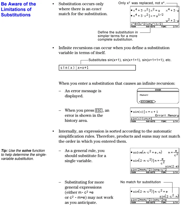 Define the substitution in simpler terms for a more complete substitution.
-
Infinite recursions can occur when you define a substitution variable in terms of itself. Substitutes \sin(x+1), \sin(x+1+1), \sin(x+1+1+1), etc.
 Define the substitution in simpler terms for a more complete substitution.
When you enter a substitution that causes an infinite recursion:
– An error message is displayed.
– When you press [ESC], an error is shown in the history area.
- Internally, an expression is sorted according to the automatic simplification rules. Therefore, products and sums may not match the order in which you entered them.
Tip: Use the solve function to help determine the single-variable substitution.
– As a general rule, you should substitute for a single variable.
– Substituting for more general expressions (either m \cdot c^2 = e or c^2 \cdot m = e) may not work as you anticipate. No match for substitution
68 Chapter 3: Symbolic Manipulation
Specifying Domain Constraints
Many identities and transformations are valid for only a particular domain. For example:
\ln(x \cdot y) = \ln(x) + \ln(y) only if $x$ and/or $y$ is not negative
\sin^-1(\sin(\theta)) = \theta only if \theta ≥ -\pi/2 and \theta ≤ \pi/2 radians
Use the "with" operator to specify the domain constraint.
Tip: Enter ln(x* y) instead of ln(xy); otherwise, xy is interpreted as a single variable named xy.
Because \ln(x \cdot y) = \ln(x) + \ln(y) is not always valid, the logarithms are not combined.

With a constraint, the identity is valid and the expression is simplified.
Tip: For ≥ or ≤, press [■] [>] or [■] [<]. You can also use [2nd] [MATH] 8 or [2nd] [CHAR] 2 to select them from a menu.
Because \sin^-1(\sin(\theta)) = \theta is not always valid, the expression is not simplified.
With a constraint, the expression can be simplified.
Using Substitutions vs. Defining a Variable
In many cases, you can achieve the same effect as a substitution by defining the variable.
However, substitution is preferable for most cases because the variable is defined only for the current calculation and does not accidentally affect later calculations.
Substituting x=1 does not affect the next calculation.
Caution: After x is defined, it can affect all calculations that involve x (until you delete x).
Storing 1→x affects the subsequent calculations.
Chapter 3: Symbolic Manipulation 69
Overview of the Algebra Menu
You can use the F2 Algebra toolbar menu to select the most commonly used algebraic functions.
The Algebra Menu
From the Home screen, press F2 to display:

Note: For a complete description of each function and its syntax, refer to Appendix A.
This menu is also available from the MATH menu. Press 2nd [MATH] and then select 9:Algebra.
70 Chapter 3: Symbolic Manipulation
| Menu Item | Description |
|---|---|
| Trig | Displays the submenu:<br>1:tExpand(<br>2:tCollect(<br>tExpand Expands trig expressions with angle sums and multiple angles.tCollect Collects the products of integer powers of trig functions into angle sums and multiple angles. tCollect is the opposite of tExpand. |
| Complex | Displays the submenu:<br>1:cSolve(<br>2:cFactor(<br>3:cZeros(<br>These are the same as solve, factor, and zeros; but they also compute complex results. |
| Extract | Displays the submenu:<br>1:getNum(<br>2:getDenom(<br>3:left(<br>4:right(<br>getNum Applies comDenom and then returns the resulting numerator.getDenom Applies comDenom and then returns the resulting denominator.left Returns the left-hand side of an equation or inequality.right Returns the right-hand side of an equation or inequality. |
Note: The left and right functions are also used to return a specified number of elements or characters from the left or right side of a list or character string.
Chapter 3: Symbolic Manipulation 71
Common Algebraic Operations
This section gives examples for some of the functions available from the \underlineF2 Algebra toolbar menu. For complete information about any function, refer to Appendix A. Some algebraic operations do not require a special function.
Adding or Dividing Polynomials
You can add or divide polynomials directly, without using a special function.
Factoring and Expanding Polynomials
Use the factor (\underlineF2 2) and expand (\underlineF2 3) functions.
factor(expression [,var]) for factoring with respect to a variable
expand(expression [,var]) for partial expansion with respect to a variable
Factor $x^5 - 1$. Then expand the result.
Notice that factor and expand perform opposite operations.
Finding Prime Factors of a Number
The factor (\underlineF2 2) function lets you do more than simply factor an algebraic polynomial.
You can find prime factors of a rational number (either an integer or a ratio of integers).
Finding Partial Expansions
With the expand (\underlineF2 3) function's optional var value, you can do a partial expansion that collects similar powers of a variable.
Do a full expansion of $(x^2 - x)$ $(y^2 - y)$ with respect to all variables.
Then do a partial expansion with respect to x.
72 Chapter 3: Symbolic Manipulation


Solving an Equation
Use the solve (F2 1) function to solve an equation for a specified variable.
solve(equation, var)
Solve x + y - 5 = 2x - 5y for x.
Notice that solve displays only the final result.
To see intermediate results, you can manually solve the equation step-by-step.
x + y - 5 = 2x - 5y
- 2x
- y
- 5
× (-) 1
Note: An operation such as - 2 X subtracts 2x from both sides.

Solving a System of Linear Equations
Consider a set of two equations with two unknowns:
2x - 3y = 4
- x + 7y = -12
To solve this system of equations, use any of the following methods.
| Method | Example |
|---|---|
| Use the solve function for a one-step solution. | solve(2x-3y=4 and -x+7y=-12,{x,y}) |
| Use the solve function with substitution (1) for step-by-step manipulation. | Refer to the preview at the beginning of this chapter, which solved for x = -8/11 and y = -20/11. |
| Use the simult function with a matrix. | Enter the coefficients as a matrix and the results as a constant column matrix. |
| Use the rref function with a matrix. | Enter the coefficients as an augmented matrix. |
Note: The simult and rref matrix functions are not on the F2 Algebra menu. Use 2nd [MATH] 4 or the Catalog.
Chapter 3: Symbolic Manipulation 73

Finding the Zeros of an Expression
Use the zeros (F2 4) function. zeros(expression, var)
Tip: For ≥ or ≤, type [■] [>] or [■] [<]. You can also use [2nd] [MATH] 8 or [2nd] [CHAR] 2 to select them from a menu.
Use the expression x * \sin(x) + \cos(x).
Find the zeros with respect to x in the interval 0 ≤ x and x ≤ 3.
Use the "with" operator to specify the interval.
Finding Proper Fractions and Common Denominators
Use the propFrac (F2 7) and comDenom (F2 6) functions. propFrac(rational expression [,var]) for proper fractions with respect to a variable
comDenom(expression [,var]) for common denominators that collect similar powers of this variable
Note: You can use comDenom with an expression, list, or matrix.
Find a proper fraction for the expression $(x^4 - 2x^2 + x) / (2x^2 + x + 4).$
Then transform the answer into a ratio of a fully expanded numerator and a fully expanded denominator.
Notice that propFrac and comDenom perform opposite operations.
In this example:
- 31x+60/8 is the remainder of $x^4-2x^2+x$ divided by $2x^2+x+4$.
- x^2/2 - x/4 - 15/8 is the quotient.
If you do this example on your TI-89 / TI-92 Plus, the propFrac function scrolls off the top of the screen.
74 Chapter 3: Symbolic Manipulation


Overview of the Calc Menu
You can use the [F3] Calc toolbar menu to select commonly used calculus functions.
The Calc Menu
From the Home screen, press [F3] to display:
F3: Calc 1:d( differentiate 2:∫( integrate 3:limit( 4:∑( sum 5:∏( product 6:fMin( 7:fMax( 8:arcLen(
This menu is also available from the MATH menu. Press [2nd] [MATH] and then select A:Calculus.
Note: For a complete description of each function and its syntax, refer to Appendix A.
Note: The d symbol for differentiate is a special symbol. It is not the same as typing the letter D on the keyboard. Use [F3] 1 or [2nd] [α].
| Menu Item | Description |
|---|---|
| d differentiate | Differentiates an expression with respect to a specified variable. |
| ∫ integrate | Integrates an expression with respect to a specified variable. |
| limit | Calculates the limit of an expression with respect to a specified variable. |
| Σ sum | Evaluates an expression at discrete variable values within a range and then calculates the sum. |
| Π product | Evaluates an expression at discrete variable values within a range and then calculates the product. |
| fMin | Finds candidate values of a specified variable that minimize an expression. |
| fMax | Finds candidate values of a specified variable that maximize an expression. |
| arcLen | Returns the arc length of an expression with respect to a specified variable. |
| taylor | Calculates a Taylor polynomial approximation to an expression with respect to a specified variable. |
| nDeriv | Calculates the numerical derivative of an expression with respect to a specified variable. |
| nInt | Calculates an integral as a floating-point number using quadrature (an approximation using weighted sums of integrand values). |
| deSolve | Symbolically solves many 1st and 2nd order differential equations, with or without initial conditions. |
Chapter 3: Symbolic Manipulation 75

Common Calculus Operations
This section gives examples for some of the functions available from the \boxedF3 Calc toolbar menu. For complete information about any calculus function, refer to Appendix A.
Integrating and Differentiating
Use the \int integrate (\boxedF3 2) and \boldsymbold differentiate (\boxedF3 1) functions.
\int (expression, var [low] [,up]) \boldsymbold (expression, var [,order])
lets you specify limits or a constant of integration
Note: You can integrate an expression only; you can differentiate an expression, list, or matrix.
Integrate x^2 * \sin(x) with respect to x.
Differentiate the answer with respect to x.
To get \boldsymbold, use \boxedF3 1 or \boxed2nd [\boldsymbold]. Do not simply type the letter D on the keyboard.
Finding a Limit
Use the limit (\boxedF3 3) function.
limit(expression, var, point [,direction])*
negative = from left positive = from right omitted or 0 = both
Note: You can find a limit for an expression, list, or matrix.
Find the limit of \sin(3x) / x as x approaches 0.
Finding a Taylor Polynomial
Use the taylor (\boxedF3 9) function.
taylor(expression, var, order [,point])
if omitted, expansion point is 0
Important: Degree-mode scaling by \pi/180 may cause calculus application results to appear in a different form.
Find a 6th order Taylor polynomial for \sin(x) with respect to x.
Store the answer as a user-defined function named y1(x).
Then graph \sin(x) and the Taylor polynomial.
Graph sin(x):Graph y1(x)
76 Chapter 3: Symbolic Manipulation

User-Defined Functions and Symbolic Manipulation
You can use a user-defined function as an argument for the TI-89 / TI-92 Plus’s built-in algebra and calculus functions.
For Information about Creating a User-Defined Function
Refer to:
- “Creating and Evaluating User-Defined Functions” in Chapter 5.
- “Graphing a Function Defined on the Home Screen” and “Graphing a Piecewise Defined Function” in Chapter 12.
- “Overview of Entering a Function” in Chapter 17.
Undefined Functions
You can use functions such as f(x), g(t), r(θ), etc., that have not been assigned a definition. These “undefined” functions yield symbolic results. For example:
Tip: To select d from the Calc toolbar menu, press F3 1 (or press 2nd [d] on the keyboard).
Use DelVar to ensure that f(x) and g(x) are not defined.
Then find the derivative of f(x)*g(x) with respect to x.
Single-Statement Functions
You can use user-defined functions consisting of a single expression. For example:
- Use STO► to create a user-defined secant function, where:
$ \sec(x) = 1/\cos(x) $
Tip: To select limit from the Calc toolbar menu, press F3 3.
Then find the limit of sec(x) as x approaches π/4.
- Use Define to create a user-defined function h(x), where:
$ h(x)=\int_0^x\sin(t)/t $
Define h(x)= ∫(sin(t)/t,t,0,x).
Tip: To select ∫ from the Calc toolbar menu, press F3 2 (or press 2nd [∫] on the keyboard). To select taylor, press F3 9.
Then find a 5th order Taylor polynomial for h(x) with respect to x.
Chapter 3: Symbolic Manipulation 77


Multi-Statement vs. Single-Statement Functions
Multi-statement user-defined functions should be used as an argument for numeric functions (such as nDeriv and nInt) only.
In some cases, you may be able to create an equivalent single-statement function. For example, consider a piecewise function with two pieces.
\begin{tabular}{ll} When: & Use expression: \ $x < 0$ & $-x$ \ x \geq 0 & 5 \cos(x) \ \end{tabular}
Tip: You can use your computer keyboard to type lengthy text and then use TI-GRAPH LINK to send it to the TI-89 / TI 92-Plus. See Chapter 18 for more information.
• If you were to create a multi-statement user-defined function with the form:
Func If x<0 Then Return -x Else Return 5cos(x) EndIf EndFunc
Define y1(x)=Func:If x<0 Then: ... :EndFunc
Tip: To select nInt from the Calc toolbar menu, press F3 B:nInt.
Then numerically integrate y1(x) with respect to x.
• Create an equivalent single-statement user-defined function.
Use the TI-89 / TI-92 Plus's built-in when function.
Define y1(x)=when(x<0, -x, 5cos(x))
Tip: To select | from the Calc toolbar menu, press F3 2 (or press 2nd [ ] on the keyboard).
Then integrate y1(x) with respect to x.
Press [ ] [ENTER] for a floating-point result.
78 Chapter 3: Symbolic Manipulation


If You Get an Out-of-Memory Error
The TI-89 / TI-92 Plus stores intermediate results in memory and then deletes them when the calculation is complete. Depending on the complexity of the calculation, the TI-89 / TI-92 Plus may run out of memory before a result can be calculated.
Freeing Up Memory
- Delete unneeded variables and/or Flash applications, particularly large-sized ones.
- Use 2nd [VAR-LINK] as described in Chapter 21 to view and delete variables and/or Flash applications.
- On the Home screen:
- Clear the history area (F1 8) or delete unneeded history pairs.
- You can also use F1 9 to reduce the number of history pairs that will be saved.
- Use MODE to set Exact/Approx = APPROXIMATE. (For results that have a large number of digits, this uses less memory than AUTO or EXACT. For results that have only a few digits, this uses more memory.)
Simplifying Problems
- Split the problem into parts.
- Split solve(a* b=0,var) into solve(a=0,var) and solve(b=0,var). Solve each part and combine the results.
- If several undefined variables occur only in a certain combination, replace that combination with a single variable.
- If m and c occur only as m* c$^2$, substitute e for m* c$^2$.
- In the expression \frac(a+b)^2 + \sqrt(a+b)^21 - (a+b)^2, substitute c for (a+b) and use \fracc^2 + \sqrtc^21 - c^2. In the solution, replace c with (a+b).
- For expressions combined over a common denominator, replace sums in denominators with unique new undefined variables.
- In the expression \fracx\sqrta^2 + b^2 + c + \fracy\sqrta^2 + b^2 + c, substitute d for \sqrta^2 + b^2 + c and use x/d + y/d. In the solution, replace d with \sqrta^2 + b^2 + c.
- Substitute known numeric values for undefined variables at an earlier stage, particularly if they are simple integers or fractions.
- Reformulate a problem to avoid fractional powers.
- Omit relatively small terms to find an approximation.
Chapter 3: Symbolic Manipulation 79
Special Constants Used in Symbolic Manipulation
The result of a calculation may include one of the special constants described in this section. In some cases, you may also need to enter a constant as part of your entry.
true, false These indicate the result of an identity or a Boolean expression.
 x=x is true for any value of x.
solve(x = x, x) true
5 > x : x < 3 false
5>3:x<3
MAIN BND AUTO FUNC 2/30
5<3 is false.
@n1 ... @n255 This notation indicates an "arbitrary integer" that represents any integer.
For @, press: TI-89: [STO>] TI-92 Plus: [2nd] R
When an arbitrary integer occurs multiple times in the same session, each occurrence is numbered consecutively. After it reaches 255, arbitrary integer consecutive numbering restarts at @n0. Use Clean Up 2:NewProb to reset to @n1.
A solution is at every integer multiple of \pi. solve(sin(x) = 0, x) x = @n1\cdot\pi solve(sin(x) = 1, x) x = 2\cdot@n2\cdot\pi + \pi/2 solve(sin(x)=1,x) MAIN BND AUTO FUNC 2/30 Both @n1 and @n2 represent any arbitrary integer, but this notation identifies separate arbitrary integers.
\infty, $e$ \infty represents infinity, and $e$ represents the constant 2.71828... (base of the natural logarithms).
For \infty, press: TI-89: [\infty] TI-92 Plus: [2nd] [\infty]
For $e$, press: TI-89: [$e^x$] TI-92 Plus: [2nd] [$e^x$]
These constants are often used in entries as well as results.
lim \left(1 + 1/n\right)^n $e$ limit((1+1/n)^n,n,\infty) MAIN BND AUTO FUNC 1/30
undef This indicates that the result is undefined.
Mathematically undefined ±\infty (undetermined sign) Non-unique limit
0/0 undef 1/0 undef lim sin(x) undef x\to\infty limit(sin(x),x,-\infty) MAIN BND AUTO FUNC 3/30
80 Chapter 3: Symbolic Manipulation
Constants and Measurement Units
4
- Preview of Constants and Measurement Units ........ 82
- Entering Constants or Units ........ 83
- Converting from One Unit to Another ........ 85
- Setting the Default Units for Displayed Results ........ 87
- Creating Your Own User-Defined Units ........ 88
- List of Pre-Defined Constants and Units ........ 89
Note: Constant and unit names always begin with an underscore _.
The UNITS dialog box lets you select the available constants or units from different categories.
This category lists constant values.
Remaining categories list available units.

Page 3 (F3) of the MODE dialog box lets you select from three systems of measurement to specify the default units for displayed results.

International system of measurements (metric or MKS) – meters, kilograms, etc.
English system – feet, pounds, etc.
Lets you select the units you want to use.
Note: You can also use getUnits() to get a list of the default units or setUnits() to set the default units. Refer to Appendix A.
By using the unit features, you can:
- Enter a unit for values in an expression, such as 6_m * 4_m or 23_m/_s * 10_s. The result is displayed in the selected default units.
- Convert values from one unit to another within the same category.
- Create your own user-defined units. These can be a combination of existing units or unique “standalone” units.
Chapter 4: Constants and Measurement Units 81
Preview of Constants and Measurement Units
Using the equation f = m* a, calculate the force when m = 5 kilograms and a = 20 meters/second². What is the force when a = 9.8 meters/second². (This is the acceleration due to gravity, which is a constant named _g). Convert the result from newtons to kilograms of force.
| Steps | TI-89 Keystrokes | TI-92 Plus Keystrokes | Display |
|---|---|---|---|
| 1. Display the MODE dialog box, Page 3. For Unit System mode, select SI for the metric system of measurements.Results are displayed according to these default units. | MODE [F3] ▸ 1ENTER |
MODE [F3] ◯ 1ENTER |
|
2. Create an acceleration unit for meters/second² named _ms2.The UNITS dialog box lets you select units from an alphabetical list of categories. You can use 2nd ◀ and 2nd ▶ to scroll one page at a time through the categories.Now, instead of re-entering _m/_s² each time you need it, you can use _ms2.Also, you can now use the UNITS dialog box to select _ms2 from the Acceleration category. |
2nd [UNITS] ◀ ▸ MENTER÷ 2nd [UNITS]◀ ▼ ▶ SENTER▲ 2 [STO▶]◆ [ _ ]2nd [a-lock] M Salpha 2 ENTER |
◆ [UNITS] ◀ ▸ MENTER÷ ◆ [UNITS]◀ ▼ ▶ SENTER▲ 2 [STO▶]2nd [ _ ]M S2 ENTER |
|
| 3. Calculate the force when m = 5 kilograms (_kg) and a = 20 meters/second² (_ms2).If you know the abbreviation for a unit, you can type it from the keyboard. | 5 ◆ [ _ ]2nd [a-lock] K Galpha × 2 0◆ [ _ ] 2nd [a-lock]M S alpha 2ENTER |
5 2nd [ _ ]K G× 2 02nd [ _ ]M S 2ENTER |
|
| 4. Using the same m, calculate the force for an acceleration due to gravity (the constant _g).For _g, you can use the pre-defined constant available from the UNITS dialog box or you can type _g. | 5 ◆ [ _ ]2nd [a-lock] K Galpha ×2nd [UNITS] ▸alpha GENTER ENTER |
5 2nd [ _ ]K G×◆ [UNITS] ◯GENTER ENTER |
|
5. Convert to kilograms of force (_kgf).2nd [▶] displays the ▸ conversion operator. |
▶ 2nd [▶] ◆ [ _ ]2nd [a-lock] K G Falpha ENTER |
◯ 2nd [▶] 2nd [ _ ]K G FENTER |
82 Chapter 4: Constants and Measurement Units

Entering Constants or Units
You can use a menu to select from a list of available constants and units, or you can type them directly from the keyboard.
From a Menu
The following shows how to select a unit, but you can use the same general procedure to select a constant.
From the Home screen:
- Type the value or expression.
- Display the UNITS dialog box. Press: TI-89: [2nd] [UNITS] TI-92 Plus: [♦] [UNITS]
Tip: Use [2nd] ⇨ and [2nd] ⇦ to scroll one page at a time through the categories.
Note: If you created a user-defined unit for an existing category (page 88), it is listed in the menu.
- Use ⇨ and ⇦ to move the cursor to the applicable category.
- To select the highlighted (default) unit, press [ENTER]. – or – To select a different unit from the category, press [◊]. Then highlight the applicable unit, and press [ENTER].

You can also move the cursor by typing the first letter of a unit.
The selected unit is placed in the entry line. Constant and unit names always begin with an underscore (_).
From the Keyboard
If you know the abbreviation that the TI-89 / TI-92 Plus uses for a particular constant or unit (refer to the list that begins on page 89), you can type it directly from the keyboard. For example:
256_m
Note: You can type units in either uppercase or lowercase characters.
The first character must be an underscore (). For , press: TI-89: [♦] [] TI-92 Plus: [2nd] []
• A space or a multiplication symbol () before the underscore is optional. For example, 256_m, 256 _m, and 256 _m are equivalent. – However, if you are adding units to a variable, you must put a space or * before the underscore. For example, x_m is treated as a variable, not as x with a unit.
Chapter 4: Constants and Measurement Units 83