Performing a Statistical Calculation
From the Data/Matrix Editor, use the \boxedF5 Calc toolbar menu to perform statistical calculations. You can analyze one-variable or two-variable statistics, or perform several types of regression analyses.
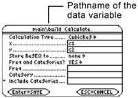
The Calculate Dialog Box
You must have a data variable opened. The Data/Matrix Editor will not perform statistical calculations with a list or matrix variable.
From the Data/Matrix Editor:
- Press \boxedF5 to display the Calculate dialog box.
This example shows all items as active. On your calculator, items are active only if they are valid for the current settings of Calculation Type and Use Freq and Categories.
Note: If an item is not valid for the current settings, it will appear dimmed. You cannot move the cursor to a dimmed item.
- Specify applicable settings for the active items.
Tip: To use an existing list variable for x, y, Freq, or Category, type the list name instead of a column number.
Chapter 16: Statistics and Data Plots 259
The Calculate Dialog Box (Continued)
| Item | Description |
|---|---|
| Freq | Type the column number that contains a “weight” value for each data point. If you do not enter a column number, all data points are assumed to have the same weight (1). |
| Category | Type the column number that contains a category value for each data point. |
| Include Categories | If you specify a Category column, you can use this item to limit the calculation to specified category values. For example, if you specify {1,4}, the calculation uses only data points with a category value of 1 or 4. |
Note: For an example of using Freq, Category, and Include Categories, refer to page 270.
- Press ENTER (after typing in an input box, press ENTER twice).
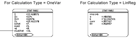
The results are displayed on the STAT VARS screen. The format depends on the Calculation Type. For example:
For Calculation Type = OneVar
When ▼ is shown instead of =, you can scroll for additional results.
For Calculation Type = LinReg
Note: Any undefined data points (shown as undef) are ignored in a stat calculation.
- To close the STAT VARS screen, press ENTER.
Redisplaying the STAT VARS Screen
The Data/Matrix Editor’s Stat toolbar menu redisplayed the previous calculation results (until they are cleared from memory).
TI-89: 2nd [F7]
TI-92 Plus: F7
Previous results are cleared when you:
• Edit the data points or change the Calculation Type.
• Open another data variable or reopen the same data variable (if the calculation referred to a column in a data variable). Results are also cleared if you leave and then reopen the Data/Matrix Editor with a data variable.
• Change the current folder (if the calculation referred to a list variable in the previous folder).
260 Chapter 16: Statistics and Data Plots
Statistical Calculation Types
As described in the previous section, the Calculate dialog box lets you specify the statistical calculation you want to perform. This section gives more information about the calculation types.
Selecting the Calculation Type
From the Calculate dialog box (F5), highlight the current setting for the Calculation Type and press ◀.
You can then select from a menu of available types.
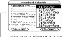
If an item is dimmed, it is not valid for the current Calculation Type.
| Calc Type | Description |
|---|---|
| OneVar | One-variable statistics — Calculates the statistical variables described on page 263. |
| TwoVar | Two-variable statistics — Calculates the statistical variables described on page 263. |
| CubicReg | Cubic regression — Fits the data to the third-order polynomial y=ax³ +bx² +cx+d. You must have at least four data points.• For four points, the equation is a polynomial fit.• For five or more points, it is a polynomial regression. |
| ExpReg | Exponential regression — Fits the data to the model equation y=ab^x (where a is the y-intercept) using a least-squares fit and transformed values x and ln(y). |
| LinReg | Linear regression — Fits the data to the model y=ax+b (where a is the slope, and b is the y-intercept) using a least-squares fit and x and y. |
| LnReg | Logarithmic regression — Fits the data to the model equation y=a+b ln(x) using a least-squares fit and transformed values ln(x) and y. |
| Logistic | Logistic regression — Fits the data to the model y=a/(1+be^(cx))+d and updates all the system statistics variables. |
Note: For TwoVar and all regression calculations, the columns that you specify for x and y (and optionally, Freq or Category) must have the same length.
Chapter 16: Statistics and Data Plots 261
Selecting the Calculation Type (Continued)
| Calc Type | Description |
|---|---|
| MedMed | Median-Median — Fits the data to the model y=ax+b (where a is the slope, and b is the y-intercept) using the median-median line, which is part of the resistant line technique.Summary points medx1, medy1, medx2, medy2, medx3, and medy3 are calculated and stored to variables, but they are not displayed on the STAT VARS screen. |
| PowerReg | Power regression — Fits the data to the model equation y=axᵇ using a least-squares fit and transformed values ln(x) and ln(y). |
| QuadReg | Quadratic regression — Fits the data to the second-order polynomial y=ax² +bx+c. You must have at least three data points.• For three points, the equation is a polynomial fit.• For four or more points, it is a polynomial regression. |
| QuartReg | Quartic regression — Fits the data to the fourth-order polynomial y=ax⁴+bx³ +cx² + dx+e. You must have at least five data points.• For five points, the equation is a polynomial fit.• For six or more points, it is a polynomial regression. |
| SinReg | Sinusoidal regression — Calculates the sinusoidal regression and updates all the system statistics variables. The output is always in radians, regardless of the angle mode setting. |
From the Home Screen or a Program
Use the applicable command for the calculation that you want to perform. The commands have the same name as the corresponding Calculation Type. Refer to Appendix A for information about each command.
Important: These commands perform a statistical calculation but do not automatically display the results. Use the ShowStat command to show the calculation results.
262 Chapter 16: Statistics and Data Plots
Statistical Variables
Statistical calculation results are stored to variables. To access these variables, type the variable name or use the VAR-LINK screen as described in Chapter 21. All statistical variables are cleared when you edit the data or change the calculation type. Other conditions that clear the variables are listed on page 260.
Calculated Variables
Statistical variables are stored as system variables. However, regCoef and regeq are treated as a list and a function variable, respectively.
To type the character \Sigma, press: TI-89: [◄] [►] [↑] [S] TI-92 Plus: [2nd] G [↑] S
To type the character \sigma, press: TI-89: [◄] [►] [alpha] [S] TI-92 Plus: [2nd] G S
Tip: To type a power (such as 2 in \Sigma x^2), \barx, or \bary, press [2nd] [CHAR] and select it from the Math menu.
Note: 1st quartile is the median of points between minX and medStat, and 3rd quartile is the median of points between medStat and maxX.
Tip: If regeq is 4x + 7, then regCoef is {4 7}. To access the "a" coefficient (the 1st element in the list), use an index such as regCoef[1].
\begin{tabular}{llll} & One Var & Two Var & Regressions \ mean of x values & \barx & \barx & \ sum of x values & \Sigma x & \Sigma x & \ sum of $x^2$ values & \Sigma x^2 & \Sigma x^2 & \ sample std. deviation of x & Sx & Sx & \ population std. deviation of x \dagger & \sigma x & \sigma x & \ number of data points & nStat & nStat & \ mean of y values & & \bary & \ sum of y values & & \Sigma y & \ sum of $y^2$ values & & \Sigma y^2 & \ sample standard deviation of y & & Sy & \ population std. deviation of y \dagger & & \sigma y & \ sum of x*y values & & \Sigma xy & \ minimum of x values & minX & minX & \ maximum of x values & maxX & maxX & \ minimum of y values & & minY & \ maximum of y values & & maxY & \ 1st quartile & q1 & & \ median & medStat & & \ 3rd quartile & q3 & & \ regression equation & & & regeq \ regression coefficients (a, b, c, d, e) & & & regCoef \ correlation coefficient \dagger\dagger & & & corr \ coefficient of determination \dagger\dagger & & & R$^2$ \ summary points (MedMed only) \dagger & & & medx1, medy1, medx2, medy2, medx3, medy3 \ \end{tabular}
\dagger The indicated variables are calculated but are not shown on the STAT VARS screen. \dagger\dagger corr is defined for a linear regression only; R$^2$ is defined for all polynomial regressions.
Chapter 16: Statistics and Data Plots 263
Defining a Statistical Plot
From the Data/Matrix Editor, you can use the entered data to define several types of statistical plots. You can define up to nine plots at a time.
Procedure
From the Data/Matrix Editor:
- Press F2 to display the Plot Setup screen.
Initially, none of the plots are defined.
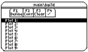
- Move the cursor to highlight the plot number that you want to define.
- Press F1 to define the plot.
This example shows all items as active. On your calculator, items are active only if they are valid for the current setting of Plot Type and Use Freq and Categories?
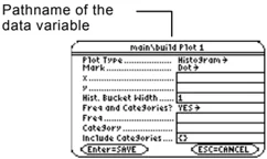
- Specify applicable settings for the active items.
Item Description Plot Type Select the type of plot. For descriptions, refer to page 266. Mark Select the symbol used to plot the data points: Box (□), Cross (x), Plus (+), Square (■), or Dot (•). x Type the column number in the Data/Matrix Editor (C1, C2, etc.) used for x values, the independent variable. y Type the column number used for y values, the dependent variable. This is active only for Plot Type = Scatter or xyline. Hist. Bucket Width Specifies the width of each bar in a histogram. For more information, refer to page 267. Use Freq and Categories? Select NO or YES. Note that Freq, Category, and Include Categories are active only when Use Freq and Categories? = YES. (Freq is active only for Plot Type = Box Plot or Histogram.)
Note: This dialog box is similar to the Calculate dialog box.
Note: If an item is not valid for the current settings, it will appear dimmed. You cannot move the cursor to a dimmed item.
Note: Plots defined with column numbers always use the last data variable in the Data/Matrix Editor, even if that variable was not used to create the definition.
Tip: To use an existing list variable for x, y, Freq, or Category, type the list name instead of the column number.
264 Chapter 16: Statistics and Data Plots
Note: For an example of using Freq, Category, and Include Categories, refer to page 270.
| Item | Description |
|---|---|
| Freq | Type the column number that contains a "weight" value for each data point. If you do not enter a column number, all data points are assumed to have the same weight (1). |
| Category | Type the column number that contains a category value for each data point. |
| Include Categories | If you specify a Category, you can use this to limit the calculation to specified category values. For example, if you specify {1,4}, the plot uses only data points with a category value of 1 or 4. |
- Press [ENTER] (after typing in an input box, press [ENTER] twice).
Note: Any undefined data points (shown as undef) are ignored in a stat plot.
The Plot Setup screen is redisplayed.
The plot you just defined is automatically selected for graphing.
Notice the shorthand definition for the plot.
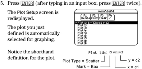
Plot 1: ☑ x=c1 y=c2 Plot Type = Scatter Mark = Box y = c2 x = c1
Selecting or Deselecting a Plot
From Plot Setup, highlight the plot and press [F4] to toggle it on or off. If a stat plot is selected, it remains selected when you:
- Change the graph mode. (Stat plots are not graphed in 3D mode.)
- Execute a Graph command.
- Open a different variable in the Data/Matrix Editor.
Copying a Plot Definition
From Plot Setup:
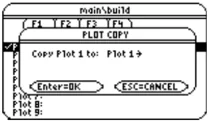
- Highlight the plot and press [F2].
Note: If the original plot was selected (✓), the copy is also selected.
-
Press [❶] and select the plot number that you want to copy to.
-
Press [ENTER].
Clearing a Plot Definition
From Plot Setup, highlight the plot and press [F3]. To redefine an existing plot, you do not necessarily need to clear it first; you can make changes to the existing definition. To prevent a plot from graphing, you can deselect it.
Chapter 16: Statistics and Data Plots 265
Statistical Plot Types
When you define a plot as described in the previous section, the Plot Setup screen lets you select the plot type. This section gives more information about the available plot types.
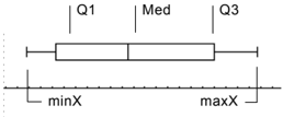
Scatter
Data points from x and y are plotted as coordinate pairs. Therefore, the columns or lists that you specify for x and y must be the same length.
- Plotted points are shown with the symbol that you select as the Mark.
- If necessary, you can specify the same column or list for both x and y.
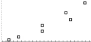
xyline
This is a scatter plot in which data points are plotted and connected in the order in which they appear in x and y.
You may want to sort all the columns in the Data/Matrix Editor before plotting.
TI-89: 2nd [F6] 3 or 2nd [F6] 4
TI-92 Plus: [F6] 3 or [F6] 4
Box Plot
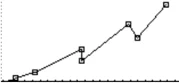
This plots one-variable data with respect to the minimum and maximum data points (minX and maxX) in the set.
- A box is defined by its first quartile (Q1), median (Med), and third quartile (Q3).
- Whiskers extend from minX to Q1 and from Q3 to maxX.
- When you select multiple box plots, they are plotted one above the other in the same order as their plot numbers.
- Use NewPlot to show statistical data as a modified box plot.
- Select Mod Box Plot as the Plot Type when you define a plot in the Data/Matrix Editor.
A modified box plot excludes points outside the interval [Q1 – X, Q3+X], where X is defined as 1.5 (Q3 – Q1). These points, called outliers, are plotted individually beyond the box plot’s whiskers, using the mark that you select.
266 Chapter 16: Statistics and Data Plots
Histogram
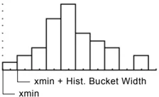
This plots one-variable data as a histogram. The x axis is divided into equal widths called buckets or bars. The height of each bar (its y value) indicates how many data points fall within the bar's range.
• When defining the plot, you can specify the Hist. Bucket Width (default is 1) to set the width of each bar.
$$ \text{Number of bars} = \frac{\text{xmax - xmin}}{\text{Hist. Bucket Width}} $$
• A data point at the edge of a bar is counted in the bar to the right.
• ZoomData (F2 9 from the Graph screen, Y= Editor, or Window Editor) adjusts xmin and xmax to include all data points, but it does not adjust the y axis. – Use [■] [WINDOW] to set ymin = 0 and ymax = the number of data points expected in the tallest bar.
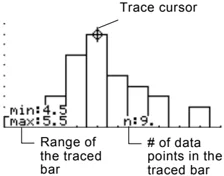
• When you trace (F3) a histogram, the screen shows information about the traced bar.
Chapter 16: Statistics and Data Plots 267

Using the Y= Editor with Stat Plots
The previous sections described how to define and select stat plots from the Data/Matrix Editor. You can also define and select stat plots from the Y= Editor.
Showing the List of Stat Plots
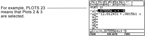
Press □ [Y=] to display the Y= Editor. Initially, the nine stat plots are located “off the top” of the screen, above the y(x) functions. However, the PLOTS indicator provides some information.
For example, PLOTS 23 means that Plots 2 & 3 are selected.
To see the list of stat plots, use ▲ to scroll above the y(x) functions.
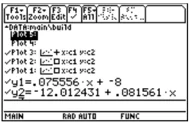
Note: Plots defined with column numbers always use the last data variable in the Data/Matrix Editor, even if that variable was not used to create the definition.
If a Plot is highlighted, this shows the data variable that will be used for the plots.
If a Plot is defined, it shows the same shorthand notation as the Plot Setup screen.
From the Y= Editor, you can perform most of the same operations on a stat plot as you can on any other y(x) function.
| To: | Do this: |
|---|---|
| Edit a plot definition | Highlight the plot and press F3. You will see the same definition screen that is displayed in the Data/Matrix Editor. |
| Select or deselect a plot | Highlight the plot and press F4. |
| Turn all plots and/or functions off | Press F5 and select the applicable item. You can also use this menu to turn all functions on. |
Note: You can not use
TI-89: 2nd [F6]
TI-92 Plus: [F6]
to set a plot’s display style. However, the plot definition lets you select the mark used for the plot.
To Graph Plots and Y= Functions
As necessary, you can select and graph stat plots and y(x) functions at the same time. The preview example at the beginning of this chapter graphs data points and their regression equations.
268 Chapter 16: Statistics and Data Plots
Graphing and Tracing a Defined Stat Plot
After entering the data points and defining the stat plots, you can graph the selected plots by using the same methods you used to graph a function from the Y= Editor (as described in Chapter 6).
Defining the Viewing Window
Stat plots are displayed on the current graph, and they use the Window variables that are defined in the Window Editor.
Use \blacklozenge [WINDOW] to display the Window Editor. You can either:
- Enter appropriate values. — or —
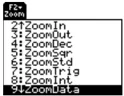
- Select 9:ZoomData from the F2 Zoom toolbar menu. (Although you can use any zoom, ZoomData is optimized for stat plots.)
Tip: F2 Zoom is available on the Y= Editor, Window Editor, and Graph screen.
ZoomData sets the viewing window to display all statistical data points.
For histograms and box plots, only xmin and xmax are adjusted. If the top of a histogram is not shown, trace the histogram to find the value for ymax.
Changing the Graph Format
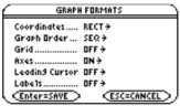
Press: F1 9 — or — TI-89: \blacklozenge | TI-92 Plus: \blacklozenge F from the Y= Editor, Window Editor, or Graph screen.
Then change the settings as necessary.
Tracing a Stat Plot
From the Graph screen, press F3 to trace a plot. The movement of the trace cursor depends on the Plot Type.
Note: When a stat plot is displayed, the Graph screen does not automatically pan if you trace off the left or right side of the screen. However, you can still press [ENTER] to center the screen on the trace cursor.
\begin{tabular}{|l|l|} \hline Plot Type & Description \ \hline Scatter or xylene & Tracing begins at the first data point. \ \hline Box plot & Tracing begins at the median. Press \blacktriangleleft to trace to Q1 and minX. Press \blacktriangleright to trace to Q3 and maxX. \ \hline Histogram & The cursor moves from the top center of each bar, starting from the leftmost bar. \ \hline \end{tabular}
When you press \blacklozenge or \blacklozenge to move to another plot or y(x) function, tracing moves to the current or beginning point on that plot (not to the nearest pixel).
Chapter 16: Statistics and Data Plots 269
Using Frequencies and Categories
To manipulate the way in which data points are analyzed, you can use frequency values and/or category values. Frequency values let you "weight" particular data points. Category values let you analyze a subset of the data points.
Example of a Frequency Column
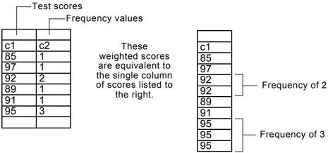
In a data variable, you can use any column in the Data/Matrix Editor to specify a frequency value (or weight) for the data points on each row. A frequency value must be an integer ≥ 0 if Calculation Type = OneVar or MedMed or if Plot Type = Box Plot. For other statistical calculations or plots, the frequency value can be any number ≥ 0.
For example, suppose you enter a student's test scores, where:
- The mid-semester exam is weighted twice as much as other tests.
- The final exam is weighted three times as much.
In the Data/Matrix Editor, you can enter the test scores and frequency values in two columns.
Tip: A frequency value of 0 effectively removes the data point from analysis.
Test scores Frequency values
c1 c2 85 1 97 1 92 2 89 1 91 1 95 3
These weighted scores are equivalent to the single column of scores listed to the right.
c1 85 97 92 92 89 91 95 95 95
Frequency of 2 Frequency of 3
Note: You can also use frequency values from a list variable instead of a column.
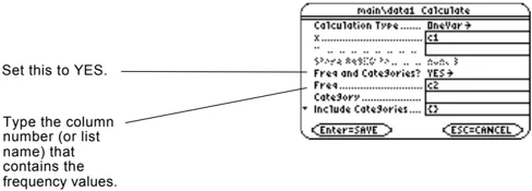
To use frequency values, specify the frequency column when you perform a statistical calculation or define a stat plot. For example:
Set this to YES.
Type the column number (or list name) that contains the frequency values.
Example of a Category Column
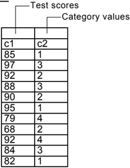
In a data variable, you can use any column to specify a category (or subset) value for the data points on each row. A category value can be any number.
270 Chapter 16: Statistics and Data Plots
Suppose you enter the test scores from a class that has 10th and 11th grade students. You want to analyze the scores for the whole class, but you also want to analyze categories such as 10th grade girls, 10th grade boys, 10th grade girls and boys, etc.
First, determine the category values you want to use.
| Category Value | Used to indicate: |
|---|---|
| 1 | 10th grade girl |
| 2 | 10th grade boy |
| 3 | 11th grade girl |
| 4 | 11th grade boy |
Note: You do not need a category value for the whole class. Also, you do not need category values for all 10th graders or all 11th graders since they are combinations of other categories.
In the Data/Matrix Editor, you can enter the scores and the category values in two columns.
To use category values, specify the category column and the category values to include in the analysis when you perform a statistical calculation or define a stat plot.
Note: You can also use category values from a list variable instead of a column.
Set this to YES.
Type the column number (or list name) that contains the category values.
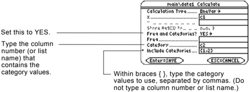
Within braces { }, type the category values to use, separated by commas. (Do not type a column number or list name.)
| To analyze: | Include Categories: |
|---|---|
| 10th grade girls | {1} |
| 10th grade boys | {2} |
| 10th grade girls and boys | {1,2} |
| 11th grade girls | {3} |
| 11th grade boys | {4} |
| 11th grade girls and boys | {3,4} |
| all girls (10th and 11th) | {1,3} |
| all boys (10th and 11th) | {2,4} |
Note: To analyze the whole class, leave the Category input box blank. Any category values are ignored.
Chapter 16: Statistics and Data Plots 271
If You Have a CBL 2/CBL or CBR
The Calculator-Based Laboratory™ System (CBL 2™/CBL™) and Calculator-Based Ranger™ System (CBR™) are optional accessories, available separately, that let you collect data from a variety of real-world experiments. TI-89 / TI-92 Plus CBL 2/CBL and CBR programs are available from the TI web site at: http://www.ti.com/calc/cbl and http://www.ti.com/calc/cbr
How CBL 2/CBL Data Is Stored
When you collect data with the CBL 2/CBL, that data is initially stored in the CBL 2/CBL unit itself. You must then retrieve the data (transfer it to the TI-89 / TI-92 Plus) by using the Get command, which is described in Appendix A.
Although each set of retrieved data can be stored in several variable types (list, real, matrix, pic), using list variables makes it easier to perform statistical calculations.
Note: For specifics about using the CBL 2/CBL and retrieving data to the TI-89 / TI-92 Plus, refer to the guidebook that comes with the CBL 2/CBL unit.
When you transfer the collected information to the TI-89 / TI-92 Plus, you can specify the list variable names that you want to use. For example, you can use the CBL 2/CBL to collect temperature data over a period of time. When you transfer the data, suppose you store:
• Temperature data in a list variable called temp.
• Time data in a list variable called time.
After you store the CBL 2/CBL information on the TI-89 / TI-92 Plus, there are two ways to use the CBL 2/CBL list variables.
Referring to the CBL 2/CBL Lists
When you perform a statistical calculation or define a plot, you can refer explicitly to the CBL 2/CBL list variables. For example:
 Type the CBL list variable name instead of a column number.
272 Chapter 16: Statistics and Data Plots
Creating a Data Variable with the CBL 2/CBL Lists
You can create a new data variable that consists of the necessary CBL 2/CBL list variables.
-
From the Home screen or a program, use the NewData command.
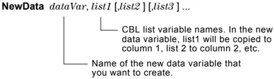
NewData dataVar, list1 [list2] [list3] ...CBL list variable names. In the new data variable, list1 will be copied to column 1, list 2 to column 2, etc.
Name of the new data variable that you want to create.
For example:
NewData temp1, time, temp
creates a data variable called temp1 in which time is in column 1 and temp is in column 2.
Tip: To define or clear a column header, use F4. For more information, refer to Chapter 15.
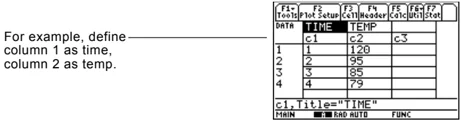
- From the Data/Matrix Editor, create a new, empty data variable with the applicable name. For each CBL 2/CBL list that you want to include, define a column header as that list name.
For example, define column 1 as time, column 2 as temp.
At this point, the columns are linked to the CBL 2/CBL lists. If the lists are changed, the columns will be updated automatically. However, if the lists are deleted, the data will be lost.
To make the data variable independent of the CBL 2/CBL lists, clear the column header for each column. The information remains in the column, but the column is no longer linked to the CBL 2/CBL list.
CBR
You can also use the Calculator-Based Ranger™(CBR™) to explore the mathematical and scientific relationships between distance, velocity, acceleration, and time using data collected from activities you perform.
Chapter 16: Statistics and Data Plots 273
274 Chapter 16: Statistics and Data Plots
Programming
17
- Preview of Programming ........ 276
- Running an Existing Program ........ 278
- Starting a Program Editor Session ........ 280
- Overview of Entering a Program ........ 282
- Overview of Entering a Function ........ 285
- Calling One Program from Another ........ 287
- Using Variables in a Program ........ 288
- Using Local Variables in Functions or Programs ........ 290
- String Operations ........ 292
- Conditional Tests ........ 294
- Using If, Lbl, and Goto to Control Program Flow ........ 295
- Using Loops to Repeat a Group of Commands ........ 297
- Configuring the TI-89 / TI-92 Plus ........ 300
- Getting Input from the User and Displaying Output ........ 301
- Creating a Custom Menu ........ 303
- Creating a Table or Graph ........ 305
- Drawing on the Graph Screen ........ 307 Accessing Another TI-89 / TI-92 Plus, a CBL 2/CBL, or a CBR ... 309
- Debugging Programs and Handling Errors ........ 310
- Example: Using Alternative Approaches ........ 311
- Assembly-Language Programs ........ 313
This chapter describes how to use the TI-89 / TI-92 Plus's Program Editor to create your own programs or functions.
Note: For details and examples of any TI-89 / TI-92 Plus program command mentioned in this chapter, refer to Appendix A.
The chapter includes:
- Specific instructions on using the Program Editor itself and running an existing program.
- An overview of fundamental programming techniques such as If...EndIf structures and various kinds of loops.
- Reference information that categorizes the available program commands.
- Obtaining and running assembly-language programs.
Chapter 17: Programming 275


Preview of Programming
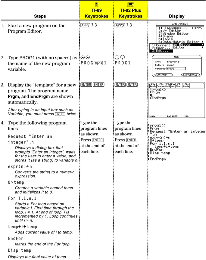
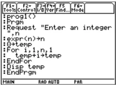
Write a program that prompts the user to enter an integer, sums all integers from 1 to the entered integer, and displays the result.
| Steps | TI-89 Keystrokes | TI-92 Plus Keystrokes | Display |
|---|---|---|---|
| 1. Start a new program on the Program Editor. | [APPS] 7 3 | [APPS] 7 3 | |
| 2. Type PROG1 (with no spaces) as the name of the new program variable. | \circ\circ P R O G [alpha] 1 | \circ\circ P R O G 1 | |
| 3. Display the “template” for a new program. The program name, Prgm, and EndPrgm are shown automatically. After typing in an input box such as Variable, you must press ENTER twice. | ENTER ENTER | ENTER ENTER | |
| 4. Type the following program lines. Request "Enter an integer",n Displays a dialog box that prompts "Enter an integer", waits for the user to enter a value, and stores it (as a string) to variable n. expr(n)\rightarrown Converts the string to a numeric expression. 0\rightarrowtemp Creates a variable named temp and initializes it to 0. For i,1,n,1 Starts a For loop based on variable i. First time through the loop, i = 1. At end of loop, i is incremented by 1. Loop continues until i > n. temp+i\rightarrowtemp Adds current value of i to temp. EndFor Marks the end of the For loop. Disp temp Displays the final value of temp. | Type the program lines as shown. Press ENTER at the end of each line. | Type the program lines as shown. Press ENTER at the end of each line. |
276 Chapter 17: Programming