FnOn [1] [, 2] ... [,99]
Selects the specified Y= functions for the current graphing mode.
Note: In 3D graphing mode, only one function at a time can be selected. FnOn 2 selects z2(x,y) and deselects any previously selected function. In the other graph modes, previously selected functions are not affected.
For CATALOG
For var, low, high [, step]
block
EndFor
Executes the statements in block iteratively for each value of var, from low to high, in increments of step.
var must not be a system variable.
step can be positive or negative. The default value is 1.
block can be either a single statement or a series of statements separated with the “:” character.
Program segment:
:0→tempsum : 1→step :For i,1,100,step : tempsum+i→tempsum :EndFor :Disp tempsum
Contents of tempsum after execution: 5050
Contents of tempsum when step is changed to 2: 2500
format() MATH/String menu
format(expression[, formatString]) ⇒ string
Returns expression as a character string based on the format template.
expression must simplify to a number.
formatString is a string and must be in the form: “F[n]”, “S[n]”, “E[n]”, “G[n][c]”, where [ ] indicate optional portions.
- F[n]: Fixed format. n is the number of digits to display after the decimal point.
- S[n]: Scientific format. n is the number of digits to display after the decimal point.
- E[n]: Engineering format. n is the number of digits after the first significant digit. The exponent is adjusted to a multiple of three, and the decimal point is moved to the right by zero, one, or two digits.
- G[n][c]: Same as fixed format but also separates digits to the left of the radix into groups of three. c specifies the group separator character and defaults to a comma. If c is a period, the radix will be shown as a comma.
- [Rc]: Any of the above specifiers may be suffixed with the Rc radix flag, where c is a single character that specifies what to substitute for the radix point.
Examples:
| Command | Output |
|---|---|
format(1.234567,"f3") ENTER |
"1.235" |
format(1.234567,"s2") ENTER |
"1.23E □" |
format(1.234567,"e3") ENTER |
"1.235E □" |
format(1.234567,"g3") ENTER |
"1.235" |
format(1234.567,"g3") ENTER |
"1,234.567" |
format(1.234567,"g3,r:") ENTER |
"1:235" |
450 Appendix A: Functions and Instructions
fpart() MATH/Number menu
fpart(expression1) \Rightarrow expression fpart(list1) \Rightarrow list fpart(matrix1) \Rightarrow matrix
Returns the fractional part of the argument.
For a list or matrix, returns the fractional parts of the elements.
The argument can be a real or a complex number.
fpart(-1.234) ENTER -.234 fpart({1, -2.3, 7.003}) ENTER {0 -.3 .003}
Func CATALOG
Func block EndFunc
Required as the first statement in a multi-statement function definition.
block can be either a single statement or a series of statements separated with the “:” character.
Note: when() also can be used to define and graph piecewise-defined functions.
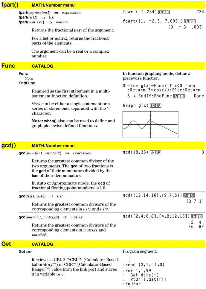
In function graphing mode, define a piecewise function:
Define g(x)=Func:If x<0 Then :Return 3*cos(x):Else:Return 3-x:EndIf:EndFunc ENTER Done
Graph g(x) ENTER
gcd() MATH/Number menu
gcd(number1, number2) \Rightarrow expression
Returns the greatest common divisor of the two arguments. The gcd of two fractions is the gcd of their numerators divided by the lcm of their denominators.
In Auto or Approximate mode, the gcd of fractional floating-point numbers is 1.0.
gcd(18,33) ENTER 3
gcd(list1, list2) \Rightarrow list
Returns the greatest common divisors of the corresponding elements in list1 and list2.
gcd({12,14,16},{9,7,5}) ENTER {3 7 1}
gcd(matrix1, matrix2) \Rightarrow matrix
Returns the greatest common divisors of the corresponding elements in matrix1 and matrix2.
gcd([2,4;6,8],[4,8;12,16]) ENTER \beginbmatrix 2 & 4 \ 6 & 8 \endbmatrix
Get CATALOG
Get var
Retrieves a CBL 2™/CBL™ (Calculator-Based Laboratory™) or CBR™ (Calculator-Based Ranger™) value from the link port and stores it in variable var.
Program segment: : :Send {3,1,-1,0} :For i,1,99 : Get data[i] : PtOn i,data[i] :EndFor :
Appendix A: Functions and Instructions 451
GetCalc CATALOG
GetCalc var
Retrieves a value from the link port and stores it in variable var. This is for unit-to-unit linking.
Note: To get a variable to the link port from another unit, use [2nd] [VAR-LINK] on the other unit to select and send a variable, or do a SendCalc on the other unit.
Program segment: :Disp "Press Enter when ready" :Pause :GetCalc L1 :Disp "List L1 received"
getConfg() CATALOG
getConfg() ⇒ ListPairs
Returns a list of calculator attributes. The attribute name is listed first, followed by its value.
TI-89: getConfg() [ENTER] {"Product Name" "Advanced Mathematics Software" "Version" "2.00, 09/25/1999" "Product ID" "03-1-4-68" "ID #" "01012 34567 ABCD" "Cert. Rev. #" □ "Screen Width" □□□ "Screen Height" □□□ "Window Width" □□□ "Window Height" □□ "RAM Size" □□□□□□ "Free RAM" □□□□□□ "Archive Size" □□□□□□ "Free Archive" 655340}
TI-92 Plus: getConfg() [ENTER] {"Product Name" "Advanced Mathematics Software" "Version" "2.00, 09/25/1999" "Product ID" "01-1-4-80" "ID #" "01012 34567 ABCD" "Cert. Rev. #" □ "Screen Width" □□□ "Screen Height" □□□ "Window Width" □□□ "Window Height" □□ "RAM Size" □□□□□□ "Free RAM" □□□□□□ "Archive Size" □□□□□□ "Free Archive" 720874}
Note: Your screen may display different attribute values. The Cert. Rev. # attribute appears only if you have purchased and installed additional software into the calculator.
getDenom() MATH/Algebra/Extract menu
getDenom(expression1) ⇒ expression
Transforms expression1 into one having a reduced common denominator, and then returns its denominator.
getDenom((x+2)/(y-3)) [ENTER] y - 3 getDenom(2/7) [ENTER] 7 getDenom(1/x+(y^2+y)/y^2) [ENTER] x • y
452 Appendix A: Functions and Instructions
getFold() CATALOG
getFold() \Rightarrow nameString Returns the name of the current folder as a string.
getFold( ) [ENTER] "main" getFold( )\rightarrowoldfoldr [ENTER] "main" oldfoldr [ENTER] "main"
getKey() CATALOG
getKey() \Rightarrow integer Returns the key code of the key pressed. Returns 0 if no key is pressed.
The prefix keys (shift \blacktriangle, second function [2nd], option \blacksquare, alpha [alpha], and drag [C]) are not recognized by themselves; however, they modify the keycodes of the key that follows them. For example: \blacksquare X \neq X \neq [2nd] X.
For a listing of key codes, see Appendix B.
Program listing: :Disp :Loop : getKey()\rightarrowkey : while key=0 : getKey()\rightarrowkey : EndWhile : Disp key : If key = ord("a") : Stop :EndLoop
getMode() CATALOG
getMode(modeNameString) \Rightarrow string getMode("ALL") \Rightarrow ListStringPairs
If the argument is a specific mode name, returns a string containing the current setting for that mode.
If the argument is "ALL", returns a list of string pairs containing the settings of all the modes. If you want to restore the mode settings later, you must store the getMode("ALL") result in a variable, and then use setMode() to restore the modes.
For a listing of mode names and possible settings, see setMode().
Note: To set or return information about the Unit System mode, use setUnits() or getUnits() instead of setMode() or getMode().
getMode("angle") [ENTER] "Radian" getMode("graph") [ENTER] "FUNCTION" getMode("all") [ENTER] {"Graph" "FUNCTION" "Display Digits" "FLOAT 6" "Angle" "Radian" "Exponential Format" "NORMAL" "Complex Format" "REAL" "Vector Format" "RECTANGULAR" "Pretty Print" "ON" "Split Screen" "FULL" "Split 1 App" "Home" "Split 2 App" "Graph" "Number of Graphs" "1" "Graph 2" "FUNCTION" "Split Screen Ratio" "1,1" "Exact/Approx" "AUTO" "Base" "DEC"}
Note: Your screen may display different mode settings.
getNum() MATH/Algebra/Extract menu
getNum(expression1) \Rightarrow expression Transforms expression1 into one having a reduced common denominator, and then returns its numerator.
getNum((x+2)/(y-3)) [ENTER] x + 2 getNum(2/7) [ENTER] 2 getNum(1/x+1/y) [ENTER] x + y
Appendix A: Functions and Instructions 453
getType() CATALOG
getType(var) ⇒ string
Returns a string indicating the data type of variable var.
If var has not been defined, returns the string "NONE".
| {1,2,3}→temp ENTER | {1 2 3} |
|---|---|
| getType(temp) ENTER | "LIST" |
| 2+3i→temp ENTER | 2 + 3i |
| getType(temp) ENTER | "EXPR" |
| DelVar temp ENTER | Done |
| getType(temp) ENTER | "NONE" |
| Data Type | Variable Contents |
|---|---|
| "ASM" | Assembly-language program |
| "DATA" | Data type |
| "EXPR" | Expression (includes complex/arbitrary/undefined, ∞, -∞, TRUE, FALSE, pi, e) |
| "FUNC" | Function |
| "GDB" | Graph data base |
| "LIST" | List |
| "MAT" | Matrix |
| "NONE" | Variable does not exist |
| "NUM" | Real number |
| "OTHER" | Miscellaneous data type for future use by software applications |
| "PIC" | Picture |
| "PRGM" | Program |
| "STR" | String |
| "TEXT" | Text type |
| "VAR" | Name of another variable |
getUnits() CATALOG
getUnits() ⇒ list
Returns a list of strings that contain the current default units for all categories except constants, temperature, amount of substance, luminous intensity, and acceleration. list has the form:
{"system" "cat1" "unit1" "cat2" "unit2" ...}
The first string gives the system (SI, ENG/US, or CUSTOM). Subsequent pairs of strings give a category (such as Length) and its default unit (such as _m for meters).
To set the default units, use setUnits().
getUnits() ENTER
{"SI" "Area" "NONE" "Capacitance" "_F" "Charge" "_coul" ... }
Note: Your screen may display different default units.
454 Appendix A: Functions and Instructions
Goto CATALOG
Goto labelName
Transfers program control to the label labelName.
labelName must be defined in the same program using a Lbl instruction.
Program segment: :0➔temp :1➔i :Lbl TOP : temp+i➔temp : If i<10 Then : i+1➔i : Goto TOP : EndIf :Disp temp :
Graph CATALOG
Graph expression1, expression2 [ , var1 ] [ , var2 ]
The Smart Graph feature graphs the requested expressions/ functions using the current graphing mode.
Expressions entered using the Graph or Table commands are assigned increasing function numbers starting with 1. They can be modified or individually deleted using the edit functions available when the table is displayed by pressing F4 Header. The currently selected Y= functions are ignored.
If you omit an optional var argument, Graph uses the independent variable of the current graphing mode.
Note: Not all optional arguments are valid in all modes because you can never have all four arguments at the same time.
Some valid variations of this instruction are:
Function graphing Graph expr, x
Parametric graphing Graph xExpr, yExpr, t
Polar graphing Graph expr, \theta
Sequence graphing Not allowed.
3D graphing Graph expr, x, y
Diff Equations graphing Not allowed.
Note: Use ClrGraph to clear these functions, or go to the Y= Editor to re-enable the system Y= functions.
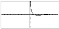
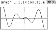
In function graphing mode and ZoomStd window: Graph 1.25a*cos(a),a ENTER
In parametric graphing mode and ZoomStd window: Graph time,2cos(time)/time,time ENTER
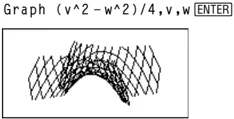
In 3D graphing mode: Graph (v^2-w^2)/4,v,w ENTER
Appendix A: Functions and Instructions 455
►Hex MATH/Base menu
integer1 ►Hex \Rightarrow integer 256►Hex [ENTER] 0h100 0b111100001111►Hex [ENTER] 0hF0F
Converts integer1 to a hexadecimal number. Binary or hexadecimal numbers always have a 0b or 0h prefix, respectively.
Zero, not the letter O, followed by b or h. 0binaryNumber 0hhexadecimalNumber
A binary number can have up to 32 digits. A hexadecimal number can have up to 8.
Without a prefix, integer1 is treated as decimal (base 10). The result is displayed in hexadecimal, regardless of the Base mode.
If you enter a decimal integer that is too large for a signed, 32-bit binary form, a symmetric modulo operation is used to bring the value into the appropriate range.
identity() MATH/Matrix menu
identity(expression) \Rightarrow matrix identity(4) [ENTER]
Returns the identity matrix with a dimension of expression.
expression must evaluate to a positive integer.
$$ \begin{bmatrix} 1 & 0 & 0 & 0 \ 0 & 1 & 0 & 0 \ 0 & 0 & 1 & 0 \ 0 & 0 & 0 & 1 \end{bmatrix} $$
If CATALOG
If Boolean expression statement If Boolean expression Then block EndIf
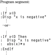
Program segment: \vdots :If x<0 :Disp "x is negative" \vdots —or— \vdots :If x<0 Then : Disp "x is negative" : abs(x)►x :EndIf \vdots
If Boolean expression evaluates to true, executes the single statement statement or the block of statements block before continuing execution.
If Boolean expression evaluates to false, continues execution without executing the statement or block of statements.
block can be either a single statement or a sequence of statements separated with the “:” character.
If Boolean expression Then block1 Else block2 EndIf
Program segment: \vdots :If x<0 Then : Disp "x is negative" : Else : Disp "x is positive or zero" :EndIf \vdots
If Boolean expression evaluates to true, executes block1 and then skips block2.
If Boolean expression evaluates to false, skips block1 but executes block2.
block1 and block2 can be a single statement.
456 Appendix A: Functions and Instructions
If Boolean expression1 Then block1 Elseif Boolean expression2 Then block2 : Elseif Boolean expressionN Then blockN EndIf
Allows for program branching. If Boolean expression1 evaluates to true, executes block1. If Boolean expression1 evaluates to false, evaluates Boolean expression2, etc.
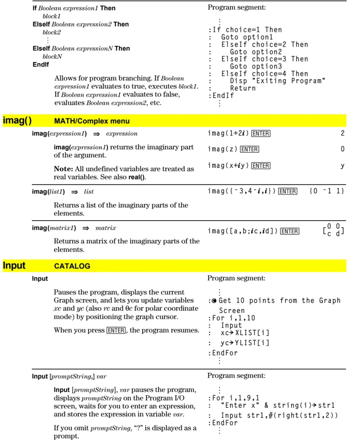
Program segment: : :If choice=1 Then : Goto option1 :ElseIf choice=2 Then : Goto option2 :ElseIf choice=3 Then : Goto option3 :ElseIf choice=4 Then : Disp "Exiting Program" : Return :EndIf :
imag() MATH/Complex menu
imag(expression1) ⇒ expression
imag(expression1) returns the imaginary part of the argument.
Note: All undefined variables are treated as real variables. See also real().
| Example | Result |
|---|---|
| imag(1+2i) ENTER | 2 |
| imag(z) ENTER | 0 |
| imag(x+iy) ENTER | y |
imag(list1) ⇒ list
Returns a list of the imaginary parts of the elements.
| Example | Result |
|---|---|
| imag({-3,4-i,i}) ENTER | {0 -1 1} |
imag(matrix1) ⇒ matrix
Returns a matrix of the imaginary parts of the elements.
| Example | Result |
|---|---|
| imag([a,b;ic,id]) ENTER | [0 0] |
| [c d] |
Input CATALOG
Input
Pauses the program, displays the current Graph screen, and lets you update variables xc and yc (also rc and θc for polar coordinate mode) by positioning the graph cursor.
When you press ENTER, the program resumes.
Program segment: : :●Get 10 points from the Graph Screen :For i,1,10 : Input : xc→XLIST[i] : yc→YLIST[i] :EndFor :
Input [promptString,] var
Input [promptString], var pauses the program, displays promptString on the Program I/O screen, waits for you to enter an expression, and stores the expression in variable var.
If you omit promptString, “?” is displayed as a prompt.
Program segment: : :For i,1,9,1 : "Enter x" & string(i)→str1 : Input str1,#(right(str1,2)) :EndFor :
Appendix A: Functions and Instructions 457
InputStr CATALOG
InputStr [promptString,] var
Pauses the program, displays promptString on the Program I/O screen, waits for you to enter a response, and stores your response as a string in variable var.
If you omit promptString, “?” is displayed as a prompt.
Note: The difference between Input and InputStr is that InputStr always stores the result as a string so that “ ” are not required.
Program segment: \vdots :InputStr "Enter Your Name",str1 \vdots
inString() MATH/String menu
inString(srcString, subString[, start]) \Rightarrow integer
Returns the character position in string srcString at which the first occurrence of string subString begins.
start, if included, specifies the character position within srcString where the search begins. Default = 1 (the first character of srcString).
If srcString does not contain subString or start is > the length of srcString, returns zero.
inString("Hello there","the") [ENTER] 7 "ABCEFG"→s1:If inString(s1, "D")=0:Disp "D not found." [ENTER] D not found.
int() CATALOG
int(expression) \Rightarrow integer int(list1) \Rightarrow list int(matrix1) \Rightarrow matrix
Returns the greatest integer that is less than or equal to the argument. This function is identical to floor().
The argument can be a real or a complex number.
For a list or matrix, returns the greatest integer of each of the elements.
int(-2.5) [ENTER] -3. int([-1.234,0,0.37]) [ENTER] [-2. 0 0.]
intDiv() CATALOG
intDiv(number1, number2) \Rightarrow integer intDiv(list1, list2) \Rightarrow list intDiv(matrix1, matrix2) \Rightarrow matrix
Returns the signed integer part of argument 1 divided by argument 2.
For lists and matrices returns the signed integer part of argument 1 divided by argument 2 for each element pair.
intDiv(-7,2) [ENTER] -3 intDiv(4,5) [ENTER] 0 intDiv({12,-14,-16},{5,4,-3}) [ENTER] {2 -3 5}
integrate See ∫(), page 532.
458 Appendix A: Functions and Instructions
iPart() MATH/Number menu
iPart(number) \Rightarrow integer iPart(list1) \Rightarrow list iPart(matrix1) \Rightarrow matrix
Returns the integer part of the argument.
For lists and matrices, returns the integer part of each element.
The argument can be a real or a complex number.
iPart(-1.234) ENTER -1. iPart({3/2,-2.3,7.003}) ENTER {1 -2. 7.}
isPrime() MATH/Test menu
isPrime(number) \Rightarrow Boolean constant expression
Returns true or false to indicate if number is a whole number \geq 2 that is evenly divisible only by itself and 1.
If number exceeds about 306 digits and has no factors \leq 1021, isPrime(number) displays an error message.
If you merely want to determine if number is prime, use isPrime() instead of factor(). It is much faster, particularly if number is not prime and has a second-largest factor that exceeds about five digits.
IsPrime(5) ENTER true IsPrime(6) ENTER false
Function to find the next prime after a specified number:
Define nextPrim(n)=Func:Loop: n+1\Rightarrown:if isPrime(n):return n: EndLoop:EndFunc ENTER Done
nextPrim(7) ENTER 11
Item CATALOG
Item itemNameString Item itemNameString, label
Valid only within a Custom...EndCustm or ToolBar...EndTBar block. Sets up a drop-down menu element to let you paste text to the cursor position (Custom) or branch to a label (ToolBar).
Note: Branching to a label is not allowed within a Custom block.
See Custom example.
Lbl CATALOG
Lbl labelName
Defines a label with the name labelName in the program.
You can use a Goto labelName instruction to transfer program control to the instruction immediately following the label.
labelName must meet the same naming requirements as a variable name.
Program segment:
: :Lbl lbl1 :InputStr "Enter password", str1 :If str1\neqpassword : Goto lbl1 :Disp "Welcome to ..." :
Appendix A: Functions and Instructions 459
lcm()
MATH/Number menu
lcm(number1, number2) ⇒ expression
lcm(list1, list2) ⇒ list
lcm(matrix1, matrix2) ⇒ matrix
Returns the least common multiple of the two arguments. The lcm of two fractions is the lcm of their numerators divided by the gcd of their denominators. The lcm of fractional floating-point numbers is their product.
For two lists or matrices, returns the least common multiples of the corresponding elements.
lcm(6,9) ENTER 18
lcm({1/3,-14,16},{2/15,7,5}) ENTER {2/3 14 80}
left()
MATH/String menu
left(sourceString[, num]) ⇒ string
Returns the leftmost num characters contained in character string sourceString.
If you omit num, returns all of sourceString.
left("Hello",2) ENTER "He"
left(list1[, num]) ⇒ list
Returns the leftmost num elements contained in list1.
If you omit num, returns all of list1.
left({1,3,-2,4},3) ENTER {1 3 -2}
left(comparison) ⇒ expression
Returns the left-hand side of an equation or inequality.
left(x<3) ENTER x
limit()
MATH/Calculus menu
limit(expression1, var, point[, direction]) ⇒ expression
limit(list1, var, point[, direction]) ⇒ list
limit(matrix1, var, point[, direction]) ⇒ matrix
Returns the limit requested.
direction: negative=from left, positive=from right, otherwise=both. (If omitted, direction defaults to both.)
limit(2x+3,x,5) ENTER 13
limit(1/x,x,0,1) ENTER ∞
limit(sin(x)/x,x,0) ENTER 1
limit((sin(x+h)-sin(x))/h,h,0) ENTER cos(x)
limit((1+1/n)^n,n,∞) ENTER e
Limits at positive ∞ and at negative ∞ are always converted to one-sided limits from the finite side.
Depending on the circumstances, limit() returns itself or undef when it cannot determine a unique limit. This does not necessarily mean that a unique limit does not exist. undef means that the result is either an unknown number with finite or infinite magnitude, or it is the entire set of such numbers.
460 Appendix A: Functions and Instructions
limit() uses methods such as L'Hopital's rule, so there are unique limits that it cannot determine. If expression1 contains undefined variables other than var, you might have to constrain them to obtain a more concise result.
Limits can be very sensitive to rounding error. When possible, avoid the APPROX setting of the Exact/Approx mode and approximate numbers when computing limits. Otherwise, limits that should be zero or have infinite magnitude probably will not, and limits that should have finite non-zero magnitude might not.
$$ \begin{aligned} & \text { limit(a^x,x, } \infty) \quad \text { ENTER } \ & \text { limit(a^x,x, } \infty) \mid a>1 \text { ENTER } \ & \text { limit(a^x,x, } \infty) \mid a>0 \text { and } a<1 \ & \text { ENTER } \end{aligned} \begin{array}{r} \text { undef } \ \infty \ 0 \end{array}
Line CATALOG
Line xStart, yStart, xEnd, yEnd[, drawMode]
Displays the Graph screen and draws, erases, or inverts a line segment between the window coordinates (xStart, yStart) and (xEnd, yEnd), including both endpoints.
If drawMode = 1, draws the line (default).
If drawMode = 0, turns off the line.
If drawMode = -1, turns a line that is on to off or off to on (inverts pixels along the line).
Note: Regraphing erases all drawn items. See also PxlLine.
In the ZoomStd window, draw a line and then erase it.
Line 0,0,6,9 ENTER
TI-89: HOME
TI-92 Plus: [icon] HOME
Line 0,0,6,9,0 ENTER
LineHorz CATALOG
LineHorz y [, drawMode]
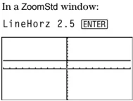
Displays the Graph screen and draws, erases, or inverts a horizontal line at window position y.
If drawMode = 1, draws the line (default).
If drawMode = 0, turns off the line.
If drawMode = -1, turns a line that is on to off or off to on (inverts pixels along the line).
Note: Regraphing erases all drawn items. See also PxlHorz.
In a ZoomStd window:
LineHorz 2.5 ENTER
Appendix A: Functions and Instructions 461
LineTan CATALOG
LineTan expression1, expression2
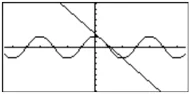
Displays the Graph screen and draws a line tangent to expression1 at the point specified.
expression1 is an expression or the name of a function, where x is assumed to be the independent variable, and expression2 is the x value of the point that is tangent.
Note: In the example shown, expression1 is graphed separately. LineTan does not graph expression1.
In function graphing mode and a ZoomTrig window:
Graph cos(x) TI-89: [HOME] TI-92 Plus: [♦] [HOME] LineTan cos(x),π/4 [ENTER]
LineVert CATALOG
LineVert x [, drawMode]
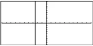
Displays the Graph screen and draws, erases, or inverts a vertical line at window position x.
If drawMode = 1, draws the line (default).
If drawMode = 0, turns off the line.
If drawMode = -1, turns a line that is on to off or off to on (inverts pixels along the line).
Note: Regraphing erases all drawn items. See also PxIVert.
In a ZoomStd window:
LineVert -2.5 [ENTER]
LinReg MATH/Statistics/Regressions menu
LinReg list1, list2[, [list3] [, list4, list5]]
Calculates the linear regression and updates all the system statistics variables.
All the lists must have equal dimensions except for list5.
list1 represents xlist.
list2 represents ylist.
list3 represents frequency.
list4 represents category codes.
list5 represents category include list.
Note: list1 through list4 must be a variable name or c1–c99 (columns in the last data variable shown in the Data/Matrix Editor). list5 does not have to be a variable name and cannot be c1–c99.
In function graphing mode:
{0,1,2,3,4,5,6}→L1 [ENTER] {0,2,3,4,3,4,6}→L2 [ENTER] LinReg L1,L2 [ENTER] ShowStat [ENTER]
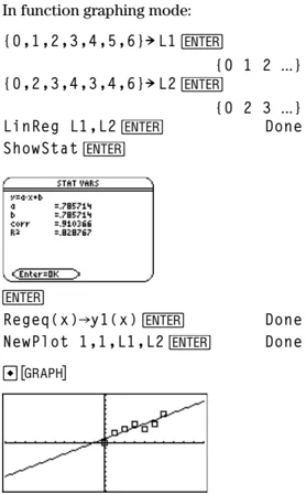
[ENTER] Regeq(x)→y1(x) [ENTER] NewPlot 1,1,L1,L2 [ENTER] [♦] [GRAPH]
462 Appendix A: Functions and Instructions
list►mat() MATH/List menu
list►mat(list [, elementsPerRow]) ⇒ matrix
Returns a matrix filled row-by-row with the elements from list.
elementsPerRow, if included, specifies the number of elements per row. Default is the number of elements in list (one row).
If list does not fill the resulting matrix, zeros are added.
Examples:
list►mat({1,2,3}) ENTER → [1 2 3]
list►mat({1,2,3,4,5},2) ENTER → \beginbmatrix 1 & 2 \ 3 & 4 \ 5 & 0 \endbmatrix
Δlist() MATH/List menu
list(list1) ⇒ list
Returns a list containing the differences between consecutive elements in list1. Each element of list1 is subtracted from the next element of list1. The resulting list is always one element shorter than the original list1.
Example:
Δlist({20,30,45,70}) ENTER → {10,15,25}
ln() TI-89: 2nd [LN] key TI-92 Plus: [LN] key
ln(expression1) ⇒ expression
ln(list1) ⇒ list
Returns the natural logarithm of the argument.
For a list, returns the natural logarithms of the elements.
Examples:
ln(2.0) ENTER → .693...
If complex format mode is REAL:
ln({-3,1.2,5}) ENTER → Error: Non-real result
If complex format mode is RECTANGULAR:
ln({-3,1.2,5}) ENTER → {ln(3) + π·i .182... ln(5)}
ln(squareMatrix1) ⇒ squareMatrix
Returns the matrix natural logarithm of squareMatrix1. This is not the same as calculating the natural logarithm of each element. For information about the calculation method, refer to cos() on.
squareMatrix1 must be diagonalizable. The result always contains floating-point numbers.
Example (In Radian angle mode and Rectangular complex format mode):
ln([1,5,3;4,2,1;6,-2,1]) ENTER → $\begin{bmatrix} 1.831...+1.734...·i & .009...-1.490...·i & ... \ .448...-.725...·i & 1.064...+.623·i & ... \ -.266...-2.083...·i & 1.124...+1.790...·i & ... \end{bmatrix}$
Appendix A: Functions and Instructions 463
LnReg
MATH/Statistics/Regressions menu
LnReg list1, list2[, [list3] [, list4, list5]]
Calculates the logarithmic regression and updates all the system statistics variables.
All the lists must have equal dimensions except for list5.
list1 represents xlist. list2 represents ylist. list3 represents frequency. list4 represents category codes. list5 represents category include list.
Note: list1 through list4 must be a variable name or c1–c99 (columns in the last data variable shown in the Data/Matrix Editor). list5 does not have to be a variable name and cannot be c1–c99.
In function graphing mode:
{1,2,3,4,5,6,7,8}→L1 ENTER {1 2 3 ...} {1,2,2,3,3,3,4,4}→L2 ENTER {1 2 2 ...} LnReg L1,L2 ENTER Done ShowStat ENTER
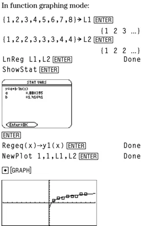
ENTER Regeq(x)→y1(x) ENTER Done NewPlot 1,1,L1,L2 ENTER Done ♦ [GRAPH]
Local
CATALOG
Local var1[, var2] [, var3] ...
Declares the specified vars as local variables. Those variables exist only during evaluation of a program or function and are deleted when the program or function finishes execution.
Note: Local variables save memory because they only exist temporarily. Also, they do not disturb any existing global variable values. Local variables must be used for For loops and for temporarily saving values in a multi-line function since modifications on global variables are not allowed in a function.
Program listing:
:prgmname() :Pr gm :Local x,y :Input "Enter x",x :Input "Enter y",y :Disp x*y :EndPrgm
Note: x and y do not exist after the program executes.
Lock
CATALOG
Lock var1[, var2] ...
Locks the specified variables. This prevents you from accidentally deleting or changing the variable without first using the unlock instruction on that variable.
In the example to the right, the variable L1 is locked and cannot be deleted or modified.
Note: The variables can be unlocked using the Unlock command.
{1,2,3,4}→L1 ENTER {1,2,3,4} Lock L1 ENTER Done DelVar L1 ENTER Error: Variable is locked or protected
464 Appendix A: Functions and Instructions
log()
CATALOG
log(expression1) ⇒ expression
log(list1) ⇒ list
Returns the base-10 logarithm of the argument.
For a list, returns the base-10 logs of the elements.
log(squareMatrix1) ⇒ squareMatrix
Returns the matrix base-10 logarithm of squareMatrix1. This is not the same as calculating the base-10 logarithm of each element. For information about the calculation method, refer to cos().
squareMatrix1 must be diagonalizable. The result always contains floating-point numbers.
log(2.0) ENTER
- 301...
If complex format mode is REAL:
log({-3,1.2,5}) ENTER
Error: Non-real result
If complex format mode is RECTANGULAR:
log({-3,1.2,5}) ENTER
{ ln(3)/ln(10) + π/ln(10)·i .079... ln(5)/ln(10) }
In Radian angle mode and Rectangular complex format mode:
log([1,5,3;4,2,1;6,-2,1]) ENTER
[ .795...+.753...·i .003...-.647...·i ... ]
[ .194...-.315...·i .462...+.270·i ... ]
[ -.115...-.904...·i .488...+.777...·i ... ]
Logistic
MATH/Statistics/Regressions menu
Logistic list1, list2 [, [iterations], [list3] [, list4, list5]]
Calculates the logistic regression and updates all the system statistics variables.
All the lists must have equal dimensions except for list5.
list1 represents xlist.
list2 represents ylist.
list3 represents frequency.
list4 represents category codes.
list5 represents category include list.
iterations specifies the maximum number of times a solution will be attempted. If omitted, 64 is used. Typically, larger values result in better accuracy but longer execution times, and vice versa.
Note: list1 through list4 must be a variable name or c1–c99 (columns in the last data variable shown in the Data/Matrix Editor). list5 does not have to be a variable name and cannot be c1–c99.
In function graphing mode:
{1,2,3,4,5,6}→L1 ENTER {1 2 3 ...}
{1,1.3,2.5,3.5,4.5,4.8}→L2
ENTER
{1 1.3 2.5 ...}
Logistic L1,L2 ENTER Done
ShowStat ENTER
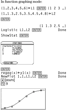
ENTER
regeq(x)→y1(x) ENTER Done
NewPlot 1,1,L1,L2 ENTER Done
◆ [GRAPH]
F2 9
Appendix A: Functions and Instructions 465
Loop CATALOG
Loop block EndLoop
Repeatedly executes the statements in block. Note that the loop will be executed endlessly, unless a Goto or Exit instruction is executed within block.
block is a sequence of statements separated with the ":" character.
Program segment: : :1→i :Loop : Rand(6)→die1 : Rand(6)→die2 : If die1=6 and die2=6 : Goto End : i+1→i :EndLoop :Lbl End :Disp "The number of rolls is", i :
LU MATH/Matrix menu
LU matrix, [lMatName, uMatName, pMatName[, tol]]
Calculates the Doolittle LU (lower-upper) decomposition of a real or complex matrix. The lower triangular matrix is stored in lMatName, the upper triangular matrix in uMatName, and the permutation matrix (which describes the row swaps done during the calculation) in pMatName.
lMatName * uMatName = pMatName * matrix
Optionally, any matrix element is treated as zero if its absolute value is less than tol. This tolerance is used only if the matrix has floating-point entries and does not contain any symbolic variables that have not been assigned a value. Otherwise, tol is ignored.
• If you use [ENTER] or set the mode to Exact/Approx=APPROXIMATE, computations are done using floating-point arithmetic.
• If tol is omitted or not used, the default tolerance is calculated as: 5\epsilon^-14 \cdot \max(\dim(matrix)) \cdot rowNorm(matrix)
The LU factorization algorithm uses partial pivoting with row interchanges.
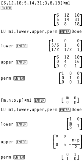
[6,12,18;5,14,31;3,8,18]→m1 [ENTER] $$ \begin{bmatrix} 6 & 12 & 18 \ 5 & 14 & 31 \ 3 & 8 & 18 \end{bmatrix} $$ LU m1,lower,upper,perm [ENTER] Done lower [ENTER] $$ \begin{bmatrix} 1 & 0 & 0 \ 5/6 & 1 & 0 \ 1/2 & 1/2 & 1 \end{bmatrix} $$ upper [ENTER] $$ \begin{bmatrix} 6 & 12 & 18 \ 0 & 4 & 16 \ 0 & 0 & 1 \end{bmatrix} $$ perm [ENTER] $$ \begin{bmatrix} 1 & 0 & 0 \ 0 & 1 & 0 \ 0 & 0 & 1 \end{bmatrix} $$ [m,n;o,p]→m1 [ENTER] $$ \begin{bmatrix} m & n \ o & p \end{bmatrix} $$ LU m1,lower,upper,perm [ENTER] Done lower [ENTER] $$ \begin{bmatrix} 1 & 0 \ m/o & 1 \end{bmatrix} $$ upper [ENTER] $$ \begin{bmatrix} o & p \ 0 & n - \frac{m \cdot p}{o} \end{bmatrix} $$ perm [ENTER] $$ \begin{bmatrix} 0 & 1 \ 1 & 0 \end{bmatrix} $$
466 Appendix A: Functions and Instructions
mat►list() MATH/List menu
mat►list(matrix) ⇒ list
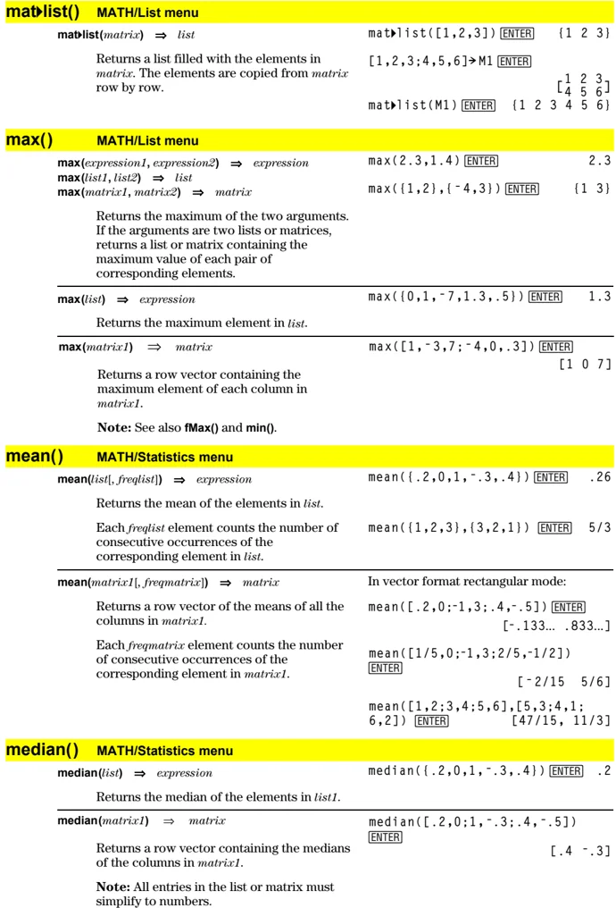
Returns a list filled with the elements in matrix. The elements are copied from matrix row by row.
mat►list([1,2,3]) ENTER {1 2 3}
[1,2,3;4,5,6]→M1 ENTER
mat►list(M1) ENTER {1 2 3 4 5 6}
max() MATH/List menu
max(expression1, expression2) ⇒ expression
max(list1, list2) ⇒ list
max(matrix1, matrix2) ⇒ matrix
Returns the maximum of the two arguments. If the arguments are two lists or matrices, returns a list or matrix containing the maximum value of each pair of corresponding elements.
max(list) ⇒ expression
Returns the maximum element in list.
max(matrix1) ⇒ matrix
Returns a row vector containing the maximum element of each column in matrix1.
Note: See also fMax() and min().
max(2.3,1.4) ENTER 2.3
max({1,2},{-4,3}) ENTER {1 3}
max({0,1,-7,1.3,.5}) ENTER 1.3
max([1,-3,7;-4,0,.3]) ENTER [1 0 7]
mean() MATH/Statistics menu
mean(list[, freqlist]) ⇒ expression
Returns the mean of the elements in list.
Each freqlist element counts the number of consecutive occurrences of the corresponding element in list.
mean(matrix1[, freqmatrix]) ⇒ matrix
Returns a row vector of the means of all the columns in matrix1.
Each freqmatrix element counts the number of consecutive occurrences of the corresponding element in matrix1.
mean({.2,0,1,-.3,.4}) ENTER .26
mean({1,2,3},{3,2,1}) ENTER 5/3
In vector format rectangular mode:
mean([.2,0;-1,3;.4,-.5]) ENTER [-.133... .833...]
mean([1/5,0;-1,3;2/5,-1/2]) ENTER [-2/15 5/6]
mean([1,2;3,4;5,6],[5,3;4,1;6,2]) ENTER [47/15, 11/3]
median() MATH/Statistics menu
median(list) ⇒ expression
Returns the median of the elements in list1.
median(matrix1) ⇒ matrix
Returns a row vector containing the medians of the columns in matrix1.
Note: All entries in the list or matrix must simplify to numbers.
median({.2,0,1,-.3,.4}) ENTER .2
median([.2,0;1,-.3;.4,-.5]) ENTER [.4 -.3]
Appendix A: Functions and Instructions 467
MedMed MATH/Statistics/Regressions menu
MedMed list1, list2[, [list3] [, list4, list5]]
Calculates the median-median line and updates all the system statistics variables.
All the lists must have equal dimensions except for list5.
list1 represents xlist. list2 represents ylist. list3 represents frequency. list4 represents category codes. list5 represents category include list.
Note: list1 through list4 must be a variable name or c1–c99 (columns in the last data variable shown in the Data/Matrix Editor). list5 does not have to be a variable name and cannot be c1–c99.
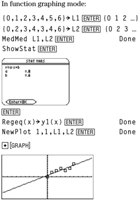
In function graphing mode:
(0,1,2,3,4,5,6)►L1 ENTER {0 1 2 ...} (0,2,3,4,3,4,6)►L2 ENTER {0 2 3 ...} MedMed L1,L2 ENTER Done ShowStat ENTER
ENTER Regeq(x)►y1(x) ENTER Done NewPlot 1,1,L1,L2 ENTER Done
mid() MATH/String menu
mid(sourceString, start[, count]) \Rightarrow string
Returns count characters from character string sourceString, beginning with character number start.
If count is omitted or is greater than the dimension of sourceString, returns all characters from sourceString, beginning with character number start.
count must be ≥ 0. If count = 0, returns an empty string.
mid("Hello there",2) ENTER "ello there" mid("Hello there",7,3) ENTER "the" mid("Hello there",1,5) ENTER "Hello" mid("Hello there",1,0) ENTER ".."
mid(sourceList, start[, count]) \Rightarrow list
Returns count elements from sourceList, beginning with element number start.
If count is omitted or is greater than the dimension of sourceList, returns all elements from sourceList, beginning with element number start.
count must be ≥ 0. If count = 0, returns an empty list.
mid({9,8,7,6},3) ENTER {7 6} mid({9,8,7,6},2,2) ENTER {8 7} mid({9,8,7,6},1,2) ENTER {9 8} mid({9,8,7,6},1,0) ENTER {}
mid(sourceStringList, start[, count]) \Rightarrow list
Returns count strings from the list of strings sourceStringList, beginning with element number start.
mid({"A","B","C","D"},2,2) ENTER {"B" "C"}
468 Appendix A: Functions and Instructions
min() MATH/List menu
min(expression1, expression2) ⇒ expression min(list1, list2) ⇒ list min(matrix1, matrix2) ⇒ matrix
Returns the minimum of the two arguments. If the arguments are two lists or matrices, returns a list or matrix containing the minimum value of each pair of corresponding elements.
min(list) ⇒ expression
Returns the minimum element of list.
min(matrix1) ⇒ matrix
Returns a row vector containing the minimum element of each column in matrix1.
Note: See also fMin() and max().
mod() MATH/Number menu
mod(expression1, expression2) ⇒ expression mod(list1, list2) ⇒ list mod(matrix1, matrix2) ⇒ matrix
Returns the first argument modulo the second argument as defined by the identities: mod(x,0) = x mod(x,y) = x - y floor(x/y)
When the second argument is non-zero, the result is periodic in that argument. The result is either zero or has the same sign as the second argument.
If the arguments are two lists or two matrices, returns a list or matrix containing the modulo of each pair of corresponding elements.
Note: See also remain().
MoveVar CATALOG
MoveVar var, oldFolder, newFolder
Moves variable var from oldFolder to newFolder. If newFolder does not exist, MoveVar creates it.
mRow() MATH/Matrix/Row ops menu
mRow(expression, matrix1, index) ⇒ matrix
Returns a copy of matrix1 with each element in row index of matrix1 multiplied by expression.
Appendix A: Functions and Instructions 469
mRowAdd() MATH/Matrix/Row ops menu
mRowAdd(expression, matrix1, index1, index2)
⇒ matrix
Returns a copy of matrix1 with each element in row index2 of matrix1 replaced with:
expression × row index1 + row index2
mRowAdd(-3,[1,2;3,4],1,2) ENTER
[ 1 2 ]
[ 0 -2 ]
mRowAdd(n,[a,b;c,d],1,2) ENTER
[ a b ]
[ a·n+c b·n+d ]
nCr() MATH/Probability menu
nCr(expression1, expression2) ⇒ expression
For integer expression1 and expression2 with expression1 ≥ expression2 ≥ 0, nCr() is the number of combinations of expression1 things taken expression2 at a time. (This is also known as a binomial coefficient.) Both arguments can be integers or symbolic expressions.
nCr(expression, 0) ⇒ 1
nCr(expression, negInteger) ⇒ 0
nCr(expression, posInteger) ⇒ expression·(expression−1)...(expression−posInteger+1)/posInteger!
nCr(expression, nonInteger) ⇒ expression!/((expression−nonInteger)!·nonInteger!)
nCr(list1, list2) ⇒ list
Returns a list of combinations based on the corresponding element pairs in the two lists. The arguments must be the same size list.
nCr({5,4,3},{2,4,2}) ENTER
{10 1 3}
nCr(matrix1, matrix2) ⇒ matrix
Returns a matrix of combinations based on the corresponding element pairs in the two matrices. The arguments must be the same size matrix.
nCr([6,5;4,3],[2,2;2,2]) ENTER
[15 10]
[ 6 3 ]
nCr(z,3)
z·(z−2)·(z−1)
─────────────
6
ans(1)|z=5
10
nCr(z,c)
z!
───────
c!(z−c)!
ans(1)/nPr(z,c)
1
──
c!
nDeriv() MATH/Calculus menu
nDeriv(expression1, var[, h]) ⇒ expression
nDeriv(expression1, var, list) ⇒ list
nDeriv(list, var[, h]) ⇒ list
nDeriv(matrix, var[, h]) ⇒ matrix
Returns the numerical derivative as an expression. Uses the central difference quotient formula.
h is the step value. If h is omitted, it defaults to 0.001.
When using list or matrix, the operation gets mapped across the values in the list or across the matrix elements.
Note: See also avgRC() and d().
nDeriv(cos(x),x,h) ENTER
-(cos(x−h)−cos(x+h))
─────────────────────
2·h
limit(nDeriv(cos(x),x,h),h,0) ENTER
-sin(x)
nDeriv(x^3,x,0.01) ENTER
3.·(x²+.000033)
nDeriv(cos(x),x)|x=π/2 ENTER
-1.
nDeriv(x^2,x,{.01,.1}) ENTER
{2.·x 2.·x}
470 Appendix A: Functions and Instructions
NewData CATALOG
NewData dataVar, list1[, list2][, list3]... Creates data variable dataVar, where the columns are the lists in order. Must have at least one list. list1, list2, ..., listn can be lists as shown, expressions that resolve to lists, or list variable names. NewData makes the new variable current in the Data/Matrix Editor.
NewData mydata,{1,2,3},{4,5,6} [ENTER] Done (Go to the Data/Matrix Editor and open the var mydata to display the data variable below.)
\begin{tabular}{|l|l|l|l|} \hline Data & c1 & c2 & c3 \ \hline 1 & 1 & 4 & \ 2 & 2 & 5 & \ 3 & 3 & 6 & \ 4 & & & \ \hline \end{tabular}
NewData dataVar, matrix Creates data variable dataVar based on matrix.
NewData sysData, matrix Loads the contents of matrix into the system data variable sysData.
NewFold CATALOG
NewFold folderName Creates a user-defined folder with the name folderName, and then sets the current folder to that folder. After you execute this instruction, you are in the new folder.
NewFold games [ENTER] Done
newList() CATALOG
newList(numElements) \Rightarrow list Returns a list with a dimension of numElements. Each element is zero.
newList(4) [ENTER] {0 0 0 0}
newMat() CATALOG also Math/Matrix menu
newMat(numRows, numColumns) \Rightarrow matrix Returns a matrix of zeros with the dimension numRows by numColumns.
newMat(2,3) [ENTER] \beginbmatrix 0 & 0 & 0 \ 0 & 0 & 0 \endbmatrix
NewPic CATALOG
NewPic matrix, picVar [, maxRow][, maxCol] Creates a pic variable picVar based on matrix. matrix must be an n × 2 matrix in which each row represents a pixel. Pixel coordinates start at 0,0. If picVar already exists, NewPic replaces it. The default for picVar is the minimum area required for the matrix values. The optional arguments, maxRow and maxCol, determine the maximum boundary limits for picVar.
NewPic [1,1;2,2;3,3;4,4;5,5; 5,1;4,2;2,4;1,5],xpic [ENTER] Done RclPic xpic [ENTER]
Appendix A: Functions and Instructions 471
NewPlot CATALOG
NewPlot n, type, xList [, yList], [frqList], [catList], [includeCatList], [mark] [, bucketSize]
Creates a new plot definition for plot number n.
type specifies the type of the graph plot. 1 = scatter plot 2 = xyline plot 3 = box plot 4 = histogram 5 = modified box plot
mark specifies the display type of the mark. 1 = □ (box) 2 = × (cross) 3 = + (plus ) 4 = ■ (square) 5 = • (dot)
bucketSize is the width of each histogram "bucket" (type = 4), and will vary based on the window variables xmin and xmax. bucketSize must be >0. Default = 1.
Note: n can be 1–9. Lists must be variable names or c1–c99 (columns in the last data variable shown in the Data/Matrix Editor), except for includeCatList, which does not have to be a variable name and cannot be c1–c99.
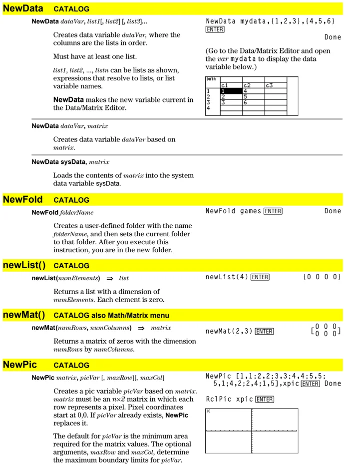
FnOff [ENTER] Done PlotsOff [ENTER] Done {1,2,3,4}►L1 [ENTER] {1 2 3 4} {2,3,4,5}►L2 [ENTER] {2 3 4 5} NewPlot 1,1,L1,L2,,,,4 [ENTER] Done
Press [GRAPH] to display:
NewProb CATALOG
NewProb
Performs a variety of operations that let you begin a new problem from a cleared state without resetting the memory.
• Clears all single-character variable names (Clear a–z) in the current folder, unless the variables are locked or archived.
• Turns off all functions and stat plots (FnOff and PlotsOff) in the current graphing mode.
• Perfoms ClrDraw, ClrErr, ClrGraph, ClrHome, ClrIO, and ClrTable.
NewProb [ENTER] Done
nInt() MATH/Calculus menu
nInt(expression1, var, lower, upper) ⇒ expression
If the integrand expression1 contains no variable other than var, and if lower and upper are constants, positive ∞, or negative ∞, then nInt() returns an approximation of ∫(expression1, var, lower, upper). This approximation is a weighted average of some sample values of the integrand in the interval lower<var<upper.
nInt(e^(-x^2),x,-1,1) [ENTER] 1.493...
472 Appendix A: Functions and Instructions
The goal is six significant digits. The adaptive algorithm terminates when it seems likely that the goal has been achieved, or when it seems unlikely that additional samples will yield a worthwhile improvement.
A warning is displayed ("Questionable accuracy") when it seems that the goal has not been achieved.
Nest nInt() to do multiple numeric integration. Integration limits can depend on integration variables outside them.
Note: See also ∫().
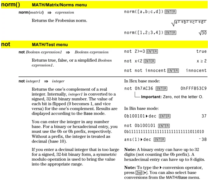
norm( ) MATH/Matrix/Norms menu
norm(matrix) \Rightarrow expression
Returns the Frobenius norm.
norm([a,b;c,d]) \boxedENTER
\sqrta^2+b^2+c^2+d^2
norm([1,2;3,4]) \boxedENTER
\sqrt30
not MATH/Test menu
not Boolean expression1 \Rightarrow Boolean expression
Returns true, false, or a simplified Boolean expression1.
not 2>=3 \boxedENTER true
not x<2 \boxedENTER x ≥ 2
not not innocent \boxedENTER innocent
not integer1 \Rightarrow integer
Returns the one's complement of a real integer. Internally, integer1 is converted to a signed, 32-bit binary number. The value of each bit is flipped (0 becomes 1, and vice versa) for the one's complement. Results are displayed according to the Base mode.
You can enter the integer in any number base. For a binary or hexadecimal entry, you must use the 0b or 0h prefix, respectively. Without a prefix, the integer is treated as decimal (base 10).
If you enter a decimal integer that is too large for a signed, 32-bit binary form, a symmetric modulo operation is used to bring the value into the appropriate range.
In Hex base mode:
not 0h7AC36 \boxedENTER 0hFFF853C9
Important: Zero, not the letter O.
In Bin base mode:
0b100101 \blacktriangleright dec \boxedENTER 37
not 0b100101 \boxedENTER
0b11111111111111111111111111011010
ans(1) \blacktriangleright dec \boxedENTER -38
Note: A binary entry can have up to 32 digits (not counting the 0b prefix). A hexadecimal entry can have up to 8 digits.
Note: To type the \blacktriangleright conversion operator, press \boxed2nd [\blacktriangleright]. You can also select base conversions from the MATH/Base menu.
Appendix A: Functions and Instructions 473
nPr() MATH/Probability menu
nPr(expression1, expression2) ⇒ expression
For integer expression1 and expression2 with expression1 ≥ expression2 ≥ 0, nPr() is the number of permutations of expression1 things taken expression2 at a time. Both arguments can be integers or symbolic expressions.
nPr(expression, 0) ⇒ 1
nPr(expression, negInteger) ⇒ 1/((expression+1)·(expression+2)...(expression−negInteger))
nPr(expression, posInteger) ⇒ expression·(expression−1)...(expression−posInteger+1)
nPr(expression, nonInteger) ⇒ expression!/(expression−nonInteger)!
nPr(list1, list2) ⇒ list
Returns a list of permutations based on the corresponding element pairs in the two lists. The arguments must be the same size list.
nPr(matrix1, matrix2) ⇒ matrix
Returns a matrix of permutations based on the corresponding element pairs in the two matrices. The arguments must be the same size matrix.
nPr(z,3) ENTER z·(z−2)·(z−1)
ans(1)|z=5 ENTER 60
nPr(z,−3) ENTER 1/((z+1)·(z+2)·(z+3))
nPr(z,c) ENTER z!/(z−c)!
ans(1)*nPr(z−c,−c) ENTER 1
nPr({5,4,3},{2,4,2}) ENTER {20 24 6}
nPr([6,5;4,3],[2,2;2,2]) ENTER [30 20; 12 6]
nSolve() MATH/Algebra menu
nSolve(equation, varOrGuess) ⇒ number or error_string
Iteratively searches for one approximate real numeric solution to equation for its one variable. Specify varOrGuess as:
variable
– or –
variable = real number
For example, x is valid and so is x=3.
nSolve() is often much faster than solve() or zeros(), particularly if the “|” operator is used to constrain the search to a small interval containing exactly one simple solution.
nSolve() attempts to determine either one point where the residual is zero or two relatively close points where the residual has opposite signs and the magnitude of the residual is not excessive. If it cannot achieve this using a modest number of sample points, it returns the string “no solution found.”
If you use nSolve() in a program, you can use getType() to check for a numeric result before using it in an algebraic expression.
Note: See also cSolve(), cZeros(), solve(), and zeros().
nSolve(x^2+5x−25=9,x) ENTER 3.844...
nSolve(x^2=4,x=−1) ENTER −2.
nSolve(x^2=4,x=1) ENTER 2.
Note: If there are multiple solutions, you can use a guess to help find a particular solution.
nSolve(x^2+5x−25=9,x)|x<0 ENTER −8.844...
nSolve(((1+r)^24−1)/r=26,r)|r>0 and r<.25 ENTER .0068...
nSolve(x^2=−1,x) ENTER "no solution found"
474 Appendix A: Functions and Instructions
OneVar MATH/Statistics menu
OneVar list1 [, list2] [, list3] [, list4]
Calculates 1-variable statistics and updates all the system statistics variables.
All the lists must have equal dimensions except for list4.
list1 represents xlist. list2 represents frequency. list3 represents category codes. list4 represents category include list.
Note: list1 through list3 must be a variable name or c1–c99 (columns in the last data variable shown in the Data/Matrix Editor). list4 does not have to be a variable name and cannot be c1–c99.
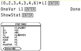
{0,2,3,4,3,4,6}→L1 [ENTER] OneVar L1 [ENTER] Done ShowStat [ENTER]
or MATH/Test menu
Boolean expression1 or Boolean expression2 ⇒ Boolean expression
Returns true or false or a simplified form of the original entry.
Returns true if either or both expressions simplify to true. Returns false only if both expressions evaluate to false.
Note: See xor.
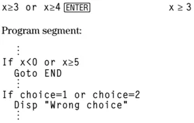
x≥3 or x≥4 [ENTER] x ≥ 3
Program segment: : If x<0 or x≥5 Goto END : If choice=1 or choice=2 Disp "Wrong choice" :
integer1 or integer2 ⇒ integer
Compares two real integers bit-by-bit using an or operation. Internally, both integers are converted to signed, 32-bit binary numbers. When corresponding bits are compared, the result is 1 if either bit is 1; the result is 0 only if both bits are 0. The returned value represents the bit results, and is displayed according to the Base mode.
You can enter the integers in any number base. For a binary or hexadecimal entry, you must use the 0b or 0h prefix, respectively. Without a prefix, integers are treated as decimal (base 10).
If you enter a decimal integer that is too large for a signed, 32-bit binary form, a symmetric modulo operation is used to bring the value into the appropriate range.
Note: See xor.
In Hex base mode: 0h7AC36 or 0h3D5F [ENTER] 0h7BD7F — Important: Zero, not the letter O.
In Bin base mode: 0b100101 or 0b100 [ENTER] 0b100101
Note: A binary entry can have up to 32 digits (not counting the 0b prefix). A hexadecimal entry can have up to 8 digits.
Appendix A: Functions and Instructions 475
ord() MATH/String menu
ord(string) ⇒ integer
ord(list1) ⇒ list
Returns the numeric code of the first character in character string string, or a list of the first characters of each list element.
See Appendix B for a complete listing of character codes.
| Command | Result |
|---|---|
ord("hello") ENTER |
104 |
char(104) ENTER |
"h" |
ord(char(24)) ENTER |
24 |
ord({"alpha","beta"}) ENTER |
{97 98} |
Output CATALOG
Output row, column, exprOrString
Displays exprOrString (an expression or character string) on the Program I/O screen at the text coordinates (row, column).
An expression can include conversion operations such as ▶DD and ▶Rect. You can also use the ▶ operator to perform unit and number base conversions.
If Pretty Print = ON, exprOrString is “pretty printed.”
From the Program I/O screen, you can press F5 to display the Home screen, or a program can use DispHome.
Program segment:
: :RandSeed 1147 :ClrIO :For i,1,90,10 : Output i, rand(100),"Hello" :EndFor :
Result after execution:
Hello Hello Hello Hello Hello Hello
P▶Rx() MATH/Angle menu
P▶Rx(rExpression, θExpression) ⇒ expression
P▶Rx(rList, θList) ⇒ list
P▶Rx(rMatrix, θMatrix) ⇒ matrix
Returns the equivalent x-coordinate of the (r, θ) pair.
Note: The θ argument is interpreted as either a degree or radian angle, according to the current angle mode. If the argument is an expression, you can use ° or ' to override the angle mode setting temporarily.
In Radian angle mode:
| Command | Result |
|---|---|
P▶Rx(r,θ) ENTER |
cos(θ)·r |
P▶Rx(4,60°) ENTER |
2 |
P▶Rx({-3,10,1.3},{π/3,-π/4,0}) ENTER |
{ -3/2 5·√2 1.3 } |
P▶Ry() MATH/Angle menu
P▶Ry(rExpression, θExpression) ⇒ expression
P▶Ry(rList, θList) ⇒ list
P▶Ry(rMatrix, θMatrix) ⇒ matrix
Returns the equivalent y-coordinate of the (r, θ) pair.
Note: The θ argument is interpreted as either a degree or radian angle, according to the current angle mode. If the argument is an expression, you can use ° or ' to override the angle mode setting temporarily.
In Radian angle mode:
| Command | Result |
|---|---|
P▶Ry(r,θ) ENTER |
sin(θ)·r |
P▶Ry(4,60°) ENTER |
2·√3 |
P▶Ry({-3,10,1.3},{π/3,-π/4,0}) ENTER |
{ -3·√3/2 -5·√2 0. } |
476 Appendix A: Functions and Instructions