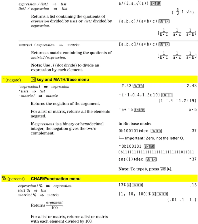
SinReg MATH/Statistics/Regressions menu
SinReg list1, list2 [, [iterations], [period] [, list3, list4]]
Calculates the sinusoidal regression and updates all the system statistics variables.
All the lists must have equal dimensions except for list4.
list1 represents xlist. list2 represents ylist. list3 represents category codes. list4 represents category include list.
iterations specifies the maximum number of times (1 through 16) a solution will be attempted. If omitted, 8 is used. Typically, larger values result in better accuracy but longer execution times, and vice versa.
period specifies an estimated period. If omitted, the difference between values in list1 should be equal and in sequential order. If you specify period, the differences between x values can be unequal.
Note: list1 through list3 must be a variable name or c1–c99 (columns in the last data variable shown in the Data/Matrix Editor). list4 does not have to be a variable name and cannot be c1–c99.
The output of SinReg is always in radians, regardless of the angle mode setting.
In function graphing mode:
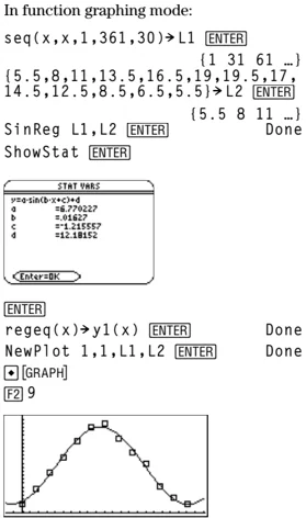
seq(x,x,1,361,30)►L1 ENTER {1 31 61 ...} {5.5,8,11,13.5,16.5,19,19.5,17, 14.5,12.5,8.5,6.5,5.5)►L2 ENTER (5.5 8 11 ...) SinReg L1,L2 ENTER Done ShowStat ENTER
ENTER regeq(x)►y1(x) ENTER Done NewPlot 1,1,L1,L2 ENTER Done [GRAPH] [F2] 9
solve() MATH/Algebra menu
solve(equation, var) \Rightarrow Boolean expression solve(inequality, var) \Rightarrow Boolean expression
Returns candidate real solutions of an equation or an inequality for var. The goal is to return candidates for all solutions. However, there might be equations or inequalities for which the number of solutions is infinite.
Solution candidates might not be real finite solutions for some combinations of values for undefined variables.
For the AUTO setting of the Exact/Approx mode, the goal is to produce exact solutions when they are concise, and supplemented by iterative searches with approximate arithmetic when exact solutions are impractical.
Due to default cancellation of the greatest common divisor from the numerator and denominator of ratios, solutions might be solutions only in the limit from one or both sides.
For inequalities of types ≥, ≤, $<$, or $>$, explicit solutions are unlikely unless the inequality is linear and contains only var.
solve(a* x^2+b* x+c=0,x) ENTER
$x = \frac\sqrtb^2-4 \cdot a \cdot c-b2 \cdot a$
or $x = \frac- (\sqrtb^2-4 \cdot a \cdot c+b)2 \cdot a$
ans(1)| a=1 and b=1 and c=1 ENTER Error: Non-real result solve((x-a)e^(x)=-x*(x-a),x) ENTER x=a or x=-.567...
(x+1)(x-1)/(x-1)+x-3 ENTER 2*x-2 solve(entry(1)=0,x) ENTER x=1 entry(2)|ans(1) ENTER undef limit(entry(3),x,1) ENTER 0 solve(5x-2≥2x,x) ENTER x≥2/3
Appendix A: Functions and Instructions 503
For the EXACT setting of the Exact/Approx mode, portions that cannot be solved are returned as an implicit equation or inequality.
Use the “|” operator to restrict the solution interval and/or other variables that occur in the equation or inequality. When you find a solution in one interval, you can use the inequality operators to exclude that interval from subsequent searches.
false is returned when no real solutions are found. true is returned if solve() can determine that any finite real value of var satisfies the equation or inequality.
Since solve() always returns a Boolean result, you can use “and,” “or,” and “not” to combine results from solve() with each other or with other Boolean expressions.
Solutions might contain a unique new undefined variable of the form @nj with j being an integer in the interval 1–255. Such variables designate an arbitrary integer.
In real mode, fractional powers having odd denominators denote only the real branch. Otherwise, multiple branched expressions such as fractional powers, logarithms, and inverse trigonometric functions denote only the principal branch. Consequently, solve() produces only solutions corresponding to that one real or principal branch.
Note: See also cSolve(), cZeros(), nSolve(), and zeros().
exact(solve((x-a)e^(x)=-x*(x-a),x)) ENTER x^e + x = 0 or x = a
In Radian angle mode: solve(tan(x)=1/x,x)|x>0 and x<1 ENTER $x = .860...$
solve(x=x+1,x) ENTER false solve(x=x,x) ENTER true
2x - 1 ≤ 1 and solve(x^2 \ne 9,x) ENTER x ≤ 1 and x \ne -3
In Radian angle mode: solve(sin(x)=0,x) ENTER x = @n1 \cdot \pi
solve(x^(1/3)=-1,x) ENTER $x = -1$ solve(\sqrtx=-2,x) ENTER false solve(-\sqrtx=-2,x) ENTER $x = 4$
solve(equation1 and equation2 [and ... ], {varOrGuess1, varOrGuess2 [, ... ]}) \Rightarrow Boolean expression
Returns candidate real solutions to the simultaneous algebraic equations, where each varOrGuess specifies a variable that you want to solve for.
Optionally, you can specify an initial guess for a variable. Each varOrGuess must have the form:
variable – or – variable = real or non-real number
For example, x is valid and so is x=3.
solve(y=x^2-2 and x+2y=-1,{x,y}) ENTER x=1 and y=-1 or x=-3/2 and y=1/4
504 Appendix A: Functions and Instructions
If all of the equations are polynomials and if you do NOT specify any initial guesses, solve() uses the lexical Gröbner/Buchberger elimination method to attempt to determine all real solutions.
For example, suppose you have a circle of radius r at the origin and another circle of radius r centered where the first circle crosses the positive x-axis. Use solve() to find the intersections.
 As illustrated by r in the example to the right, simultaneous polynomial equations can have extra variables that have no values, but represent given numeric values that could be substituted later.
You can also (or instead) include solution variables that do not appear in the equations. For example, you can include z as a solution variable to extend the previous example to two parallel intersecting cylinders of radius r.
The cylinder solutions illustrate how families of solutions might contain arbitrary constants of the form @k, where k is an integer suffix from 1 through 255. The suffix resets to 1 when you use ClrHome or [F1] 8:Clear Home.
For polynomial systems, computation time or memory exhaustion may depend strongly on the order in which you list solution variables. If your initial choice exhausts memory or your patience, try rearranging the variables in the equations and/or varOrGuess list.
If you do not include any guesses and if any equation is non-polynomial in any variable but all equations are linear in the solution variables, solve() uses Gaussian elimination to attempt to determine all real solutions.
If a system is neither polynomial in all of its variables nor linear in its solution variables, solve() determines at most one solution using an approximate iterative method. To do so, the number of solution variables must equal the number of equations, and all other variables in the equations must simplify to numbers.
solve(x^2+y^2=r^2 and (x-r)^2+y^2=r^2,{x,y}) [ENTER] $x=r/2 and y=\frac\sqrt3\cdot r2$ $ or x=r/2 and y=\frac-\sqrt3\cdot r2$
solve(x^2+y^2=r^2 and (x-r)^2+y^2=r^2,{x,y,z}) [ENTER] $x=r/2 and y=\frac\sqrt3\cdot r2 and z=@1$ $ or x=r/2 and y=\frac-\sqrt3\cdot r2 and z=@1$
solve(x+e^(z)*y=1 and x-y=sin(z),{x,y}) [ENTER] $x=e^z\cdot\sin(z)+1/e^z+1 and y=-(\sin(z)-1)/e^z+1$
solve(e^(z)*y=1 and -y=sin(z),{y,z}) [ENTER] $y=.041... and z=3.183...$
Appendix A: Functions and Instructions 505
Each solution variable starts at its guessed value if there is one; otherwise, it starts at 0.0.
Use guesses to seek additional solutions one by one. For convergence, a guess may have to be rather close to a solution.
solve(e^(z)*y=1 and -y=sin(z),{y,z=2π}) ENTER
y=.001... and z=6.281...
SortA MATH/List menu
SortA listName1[, listName2] [, listName3] ... SortA vectorName1[, vectorName2] [, vectorName3] ...
Sorts the elements of the first argument in ascending order.
If you include additional arguments, sorts the elements of each so that their new positions match the new positions of the elements in the first argument.
All arguments must be names of lists or vectors. All arguments must have equal dimensions.
{2,1,4,3}→list1 ENTER {2,1,4,3}
SortA list1 ENTER Done
list1 ENTER {1 2 3 4}
{4,3,2,1}→list2 ENTER {4 3 2 1}
SortA list2,list1 ENTER Done
list2 ENTER {1 2 3 4}
list1 ENTER {4 3 2 1}
SortD MATH/List menu
SortD listName1[, listName2] [, listName3] ... SortD vectorName1[,vectorName2] [,vectorName3] ...
Identical to SortA, except SortD sorts the elements in descending order.
{2,1,4,3}→list1 ENTER {2 1 4 3}
{1,2,3,4}→list2 ENTER {1 2 3 4}
SortD list1,list2 ENTER Done
list1 ENTER {4 3 2 1}
list2 ENTER {3 4 1 2}
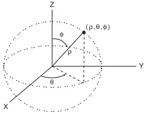
▶Sphere MATH/Matrix/Vector ops menu
vector ▶Sphere
Displays the row or column vector in spherical form [ρ ∠θ ∠φ].
vector must be of dimension 3 and can be either a row or a column vector.
Note: ▶Sphere is a display-format instruction, not a conversion function. You can use it only at the end of an entry line.
[1,2,3]▶Sphere
♦ ENTER [3.741... ∠1.107... ∠.640...]
[2,∠π/4,3]▶Sphere
♦ ENTER [3.605... ∠.785... ∠.588...]
ENTER [√13 ∠π/4 ∠cos⁻¹(3·√□□/□□)]
stdDev() MATH/Statistics menu
stdDev(list[, freqlist]) ⇒ expression
Returns the standard deviation of the elements in list.
Each freqlist element counts the number of consecutive occurrences of the corresponding element in list.
Note: list must have at least two elements.
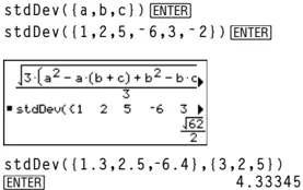
stdDev({a,b,c}) ENTER
stdDev({1,2,5,-6,3,-2}) ENTER
[√(3·(a²-a·(b+c)+b²-b·c)/3]
■ stdDev({1 2 5 -6 3 ▶
√62
2
stdDev({1.3,2.5,-6.4},{3,2,5})
ENTER 4.33345
506 Appendix A: Functions and Instructions
stdDev(matrix1[, freqmatrix]) \Rightarrow matrix
Returns a row vector of the standard deviations of the columns in matrix1.
Each freqmatrix element counts the number of consecutive occurrences of the corresponding element in matrix1.
Note: matrix1 must have at least two rows.
$$ \begin{aligned} & \text { stdDev([1,2,5;-3,0,1;.5,.7,3]) } \ & \boxed{\text { ENTER }} \quad[2.179 \ldots 1.014 \ldots 2] \ & \text { stdDev([-1.2,5.3;2.5,7.3;6,-4], } \ & {[4,2 ; 3,3 ; 1,7)]} \quad \boxed{\text { ENTER }} \quad[2.7005,5.44695] \end{aligned} $$
StoGDB CATALOG
StoGDB GDBvar
Creates a Graph database (GDB) variable that contains the current:
- Graphing mode
- Y= functions
- Window variables
- Graph format settings
- 1- or 2-Graph setting (split screen and ratio settings if 2-Graph mode)
- Angle mode
- Real/complex mode
- Initial conditions if Sequence or Diff Equations mode
- Table flags
- tblStart, \Deltatbl, tblInput
You can use RclGDB GDBvar to restore the graph environment.
*Note: These items are saved for both graphs in 2-Graph mode.
Stop CATALOG
Stop
Used as a program instruction to stop program execution.
Program segment: \vdots For i,1,10,1 If i=5 Stop EndFor \vdots
StoPic CATALOG
StoPic picVar [, pxlRow, pxlCol] [, width, height]
Displays the graph screen and copies a rectangular area of the display to the variable picVar.
pxlRow and pxlCol, if included, specify the upper-left corner of the area to copy (defaults are 0, 0).
width and height, if included, specify the dimensions, in pixels, of the area. Defaults are the width and height, in pixels, of the current graph screen.
Store See \rightarrow (store), page 539.
Appendix A: Functions and Instructions 507
string() MATH/String menu
string(expression) \Rightarrow string
Simplifies expression and returns the result as a character string.
string(1.2345) [ENTER] "1.2345" string(1+2) [ENTER] "3" string(cos(x)+√(3)) [ENTER] "cos(x) + √(3)"
Style CATALOG
Style equanum, stylePropertyString
Sets the system graphing function equanum in the current graph mode to use the graphing property stylePropertyString.
equanum must be an integer from 1–99 and the function must already exist.
stylePropertyString must be one of: "Line", "Dot", "Square", "Thick", "Animate", "Path", "Above", or "Below".
Note that in parametric graphing, only the xt half of the pair contains the style information.
Valid style names vs. graphing mode:
Function: all styles Parametric/Polar: line, dot, square, thick, animate, path Sequence: line, dot, square, thick 3D: none Diff Equations: line, dot, square, thick, animate, path
Note: Capitalization and blank spaces are optional when entering stylePropertyString names.
Style 1,"thick" [ENTER] Done Style 10,"path" [ENTER] Done
Note: In function graphing mode, these examples set the style of y1(x) to "Thick" and y10(x) to "Path".
subMat() CATALOG
subMat(matrix1[, startRow][, startCol][, endRow] [, endCol]) \Rightarrow matrix
Returns the specified submatrix of matrix1.
Defaults: startRow=1, startCol=1, endRow=last row, endCol=last column.
[1,2,3;4,5,6;7,8,9]\rightharpoonupm1 [ENTER] $ \beginbmatrix 1 & 2 & 3 \ 4 & 5 & 6 \ 7 & 8 & 9 \endbmatrix $
subMat(m1,2,1,3,2) [ENTER] $ \beginbmatrix 4 & 5 \ 7 & 8 \endbmatrix $
subMat(m1,2,2) [ENTER] $ \beginbmatrix 5 & 6 \ 8 & 9 \endbmatrix $
sum() MATH/List menu
sum(list[, start[, end]]) \Rightarrow expression
Returns the sum of the elements in list.
Start and end are optional. They specify a range of elements.
sum({1,2,3,4,5}) [ENTER] 15 sum({a,2a,3a}) [ENTER] 6·a sum(seq(n,n,1,10)) [ENTER] 55 sum({1,3,5,7,9},3) [ENTER] 21
508 Appendix A: Functions and Instructions
sum(matrix1[, start[, end]]) \Rightarrow matrix
Returns a row vector containing the sums of the elements in the columns in matrix1.
Start and end are optional. They specify a range of rows.
$$ \begin{aligned} &\text{sum}([1,2,3;4,5,6]) \boxed{\text{ENTER}} [5 \quad 7 \quad 9] \ &\text{sum}([1,2,3;4,5,6;7,8,9]) \boxed{\text{ENTER}} \ &\qquad\qquad\qquad\qquad\qquad [12 \ 15 \ 18] \ &\text{sum}([1,2,3;4,5,6;7,8,9],2,3) \ &\boxed{\text{ENTER}} \ &\qquad\qquad\qquad\qquad\qquad [11,13,15] \end{aligned} $$
switch() CATALOG
switch([integer1]) \Rightarrow integer
Returns the number of the active window. Also can set the active window.
Note: Window 1 is left or top; Window 2 is right or bottom.
If integer1 = 0, returns the active window number.
If integer1 = 1, activates window 1 and returns the previously active window number.
If integer1 = 2, activates window 2 and returns the previously active window number.
If integer1 is omitted, switches windows and returns the previously active window number.
integer1 is ignored if the TI-89 / TI-92 Plus is not displaying a split screen.
switch( ) \boxedENTER
T (transpose) MATH/Matrix menu
matrix1$^T$ \Rightarrow matrix
Returns the complex conjugate transpose of matrix1.
$$ \begin{aligned} &[1,2,3;4,5,6;7,8,9]\rightarrow\text{mat1 } \boxed{\text{ENTER}} & \begin{bmatrix} 1 & 2 & 3 \ 4 & 5 & 6 \ 7 & 8 & 9 \end{bmatrix} \ &\text{mat1}^T \boxed{\text{ENTER}} & \begin{bmatrix} 1 & 4 & 7 \ 2 & 5 & 8 \ 3 & 6 & 9 \end{bmatrix} \ &[a,b;c,d]\rightarrow\text{mat2 } \boxed{\text{ENTER}} & \begin{bmatrix} a & b \ c & d \end{bmatrix} \ &\text{mat2}^T \boxed{\text{ENTER}} & \begin{bmatrix} a & c \ b & d \end{bmatrix} \ &[1+i,2+i;3+i,4+i]\rightarrow\text{mat3 } \boxed{\text{ENTER}} & \begin{bmatrix} 1+i & 2+i \ 3+i & 4+i \end{bmatrix} \ &\text{mat3}^T \boxed{\text{ENTER}} & \begin{bmatrix} 1-i & 3-i \ 2-i & 4-i \end{bmatrix} \end{aligned} $$
Appendix A: Functions and Instructions 509
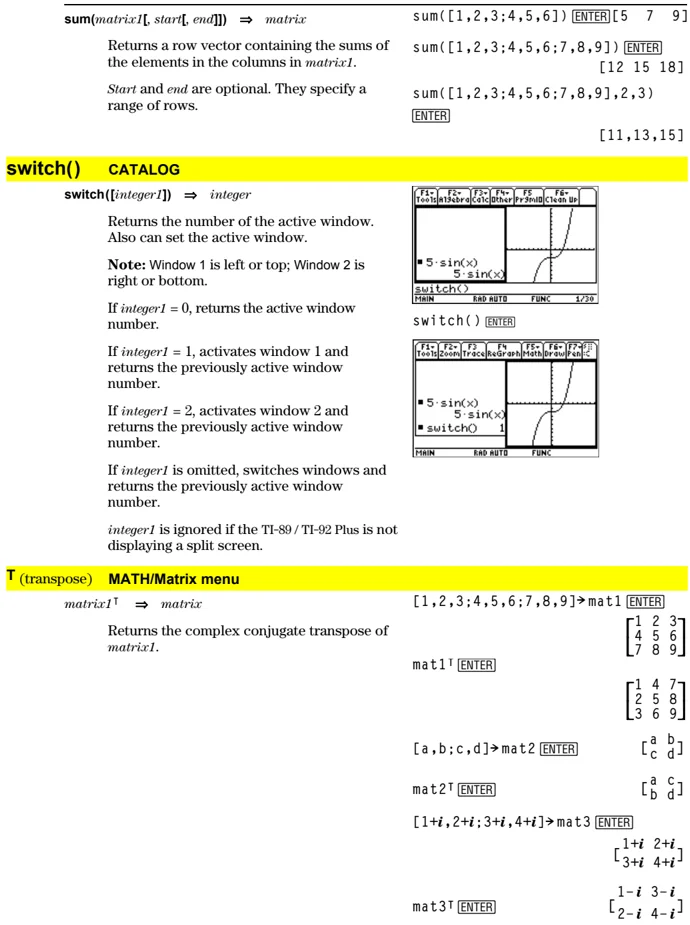
Table CATALOG
Table expression1[, expression2][, var1]
Builds a table of the specified expressions or functions.
The expressions in the table can also be graphed. Expressions entered using the Table or Graph commands are assigned increasing function numbers starting with 1. The expressions can be modified or individually deleted using the edit functions available when the table is displayed by pressing [F4] Header. The currently selected functions in the Y= Editor are temporarily ignored.
To clear the functions created by Table or Graph, execute the ClrGraph command or display the Y= Editor.
If the var parameter is omitted, the current graph-mode independent variable is assumed. Some valid variations of this instruction are:
- Function graphing:
Table expr, x - Parametric graphing:
Table xExpr, yExpr, t - Polar graphing:
Table expr, θ
Note: The Table command is not valid for 3D, sequence, or diff equations graphing. As an alternative, you may want to use BldData.
In function graphing mode.
Table 1.25x*cos(x) [ENTER]
| x | 1 | ||
|---|---|---|---|
| 0. | 0. | ||
| 1. | .67538 | ||
| 2. | -1.04 | ||
| 3. | -3.712 | ||
| 4. | -3.268 |
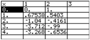
Table cos(time),time [ENTER]
| x | 1 | 2 | 3 |
|---|---|---|---|
| 0. | 0. | 1. | |
| 1. | .67538 | .5403 | |
| 2. | -1.04 | -.4161 | |
| 3. | -3.712 | -.99 | |
| 4. | -3.268 | -.6536 |
tan()
TI-89: [2nd] [TAN] key
TI-92 Plus: [TAN] key
tan(expression1) ⇒ expression
tan(list1) ⇒ list
tan(expression1) returns the tangent of the argument as an expression.
tan(list1) returns a list of the tangents of all elements in list1.
Note: The argument is interpreted as either a degree or radian angle, according to the current angle mode. You can use ° or ' to override the angle mode temporarily.
In Degree angle mode:
tan((π/4)') [ENTER] 1 tan(45) [ENTER] 1 tan({0,60,90}) [ENTER] {0 √3 undef}
In Radian angle mode:
tan(π/4) [ENTER] 1 tan(45°) [ENTER] 1 tan({π,π/3,-π,π/4}) [ENTER] {0 √3 0 1}
tan(squareMatrix1) ⇒ squareMatrix
Returns the matrix tangent of squareMatrix1. This is not the same as calculating the tangent of each element. For information about the calculation method, refer to cos().
squareMatrix1 must be diagonalizable. The result always contains floating-point numbers.
In Radian angle mode:
tan([1,5,3;4,2,1;6,-2,1]) [ENTER]
[ -28.291... 26.088... 11.114... ] [ 12.117... -7.835... -5.481... ] [ 36.818... -32.806... -10.459... ]
510 Appendix A: Functions and Instructions
tan⁻¹()
TI-89: ◻ [TAN⁻¹] key
TI-92 Plus: [2nd] [TAN⁻¹] key
tan⁻¹(expression1) ⇒ expression
tan⁻¹(list1) ⇒ list
tan⁻¹(expression1) returns the angle whose tangent is expression1 as an expression.
tan⁻¹(list1) returns a list of the inverse tangents of each element of list1.
Note: The result is returned as either a degree or radian angle, according to the current angle mode setting.
In Degree angle mode:
tan⁻¹(1) ENTER
45
In Radian angle mode:
tan⁻¹({0,.2,.5}) ENTER
{0 .197... .463...}
tan⁻¹(squareMatrix1) ⇒ squareMatrix
Returns the matrix inverse tangent of squareMatrix1. This is not the same as calculating the inverse tangent of each element. For information about the calculation method, refer to cos().
squareMatrix1 must be diagonalizable. The result always contains floating-point numbers.
In Radian angle mode:
tan⁻¹([1,5,3;4,2,1;6,-2,1])
ENTER
[ -.083... 1.266... .622... ] [ .748... .630... -.070... ] [ 1.686... -1.182... .455... ]
tanh()
MATH/Hyperbolic menu
tanh(expression1) ⇒ expression
tanh(list1) ⇒ list
tanh(expression1) returns the hyperbolic tangent of the argument as an expression.
tanh(list) returns a list of the hyperbolic tangents of each element of list1.
In Radian angle mode:
tanh(1.2) ENTER
- 833...
tanh({0,1}) ENTER
{0 tanh(1)}
tanh(squareMatrix1) ⇒ squareMatrix
Returns the matrix hyperbolic tangent of squareMatrix1. This is not the same as calculating the hyperbolic tangent of each element. For information about the calculation method, refer to cos().
squareMatrix1 must be diagonalizable. The result always contains floating-point numbers.
In Radian angle mode:
tanh([1,5,3;4,2,1;6,-2,1])
ENTER
[ -.097... .933... .425... ] [ .488... .538... -.129... ] [ 1.282... -1.034... .428... ]
tanh⁻¹()
MATH/Hyperbolic menu
tanh⁻¹(expression1) ⇒ expression
tanh⁻¹(list1) ⇒ list
tanh⁻¹(expression1) returns the inverse hyperbolic tangent of the argument as an expression.
tanh⁻¹(list1) returns a list of the inverse hyperbolic tangents of each element of list1.
In rectangular complex format mode:
tanh⁻¹(0) ENTER
0
tanh⁻¹({1,2.1,3}) ENTER
{∞ .518... - 1.570...·i ln(2)/2 · π/2 · i}
Appendix A: Functions and Instructions 511
tanh⁻¹(squareMatrix1) ⇒ squareMatrix
Returns the matrix inverse hyperbolic tangent of squareMatrix1. This is not the same as calculating the inverse hyperbolic tangent of each element. For information about the calculation method, refer to cos().
squareMatrix1 must be diagonalizable. The result always contains floating-point numbers.
In Radian angle mode and Rectangular complex format mode: tanh⁻¹([1,5,3;4,2,1;6,-2,1]) ENTER [ -.099...+.164...*i .267...-1.490...*i ... ] [ -.087...-.725...*i .479...-.947...*i ... ] [ .511...-2.083...*i -.878...+1.790...*i ... ]
taylor() MATH\Calculus menu
taylor(expression1, var, order[, point]) ⇒ expression
Returns the requested Taylor polynomial. The polynomial includes non-zero terms of integer degrees from zero through order in (var minus point). taylor() returns itself if there is no truncated power series of this order, or if it would require negative or fractional exponents. Use substitution and/or temporary multiplication by a power of (var minus point) to determine more general power series.
point defaults to zero and is the expansion point.
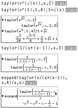
 taylor(e^(√(x)),x,2) ENTER
taylor(e^(t),t,4)| t=√(x) ENTER
■ taylor(e^√x,x,2) taylor(e^√x,x,2,0) ■ taylor(e^t,t,4)| t=√x x²/24 + x^(3/2)/6 + x/2 + √x + 1
taylor(1/(x*(x-1)),x,3) ENTER
■ taylor(1/(x·(x-1)),x,3) taylor(1/(x·(x-1)),x,3,0)
expand(taylor(x/(x*(x-1)),x,4)/x,x) ENTER
■ expand(taylor(x/(x·(x-1)),x,4)/x) -x³-x²-x-1/x-1
tCollect() MATH\Algebra\Trig menu
tCollect(expression1) ⇒ expression
Returns an expression in which products and integer powers of sines and cosines are converted to a linear combination of sines and cosines of multiple angles, angle sums, and angle differences. The transformation converts trigonometric polynomials into a linear combination of their harmonics.
Sometimes tCollect() will accomplish your goals when the default trigonometric simplification does not. tCollect() tends to reverse transformations done by tExpand(). Sometimes applying tExpand() to a result from tCollect(), or vice versa, in two separate steps simplifies an expression.
tCollect((cos(α))²) ENTER cos(2·α) + 1 / 2
tCollect(sin(α)cos(β)) ENTER sin(α-β)+sin(α+β) / 2
512 Appendix A: Functions and Instructions
tExpand() MATH\Algebra\Trig menu
tExpand(expression1) \Rightarrow expression
Returns an expression in which sines and cosines of integer-multiple angles, angle sums, and angle differences are expanded. Because of the identity (sin(x))$^2$+(cos(x))$^2$=1, there are many possible equivalent results. Consequently, a result might differ from a result shown in other publications.
Sometimes tExpand() will accomplish your goals when the default trigonometric simplification does not. tExpand() tends to reverse transformations done by tCollect(). Sometimes applying tCollect() to a result from tExpand(), or vice versa, in two separate steps simplifies an expression.
Note: Degree-mode scaling by \pi/180 interferes with the ability of tExpand() to recognize expandable forms. For best results, tExpand() should be used in Radian mode.
tExpand(sin(3\phi)) ENTER 4\cdotsin(\phi)\cdot(cos(\phi))$^2$-sin(\phi)
tExpand(cos(\alpha-\beta)) ENTER cos(\alpha)\cdotcos(\beta)+sin(\alpha)\cdotsin(\beta)
Text CATALOG
Text promptString
Displays the character string promptString dialog box.
If used as part of a Dialog...EndDlog block, promptString is displayed inside that dialog box. If used as a standalone instruction, Text creates a dialog box to display the string.
Text "Have a nice day." ENTER Done
Then See If, page 456.
Title CATALOG
Title titleString, [Lbl]
Creates the title of a pull-down menu or dialog box when used inside a Toolbar or Custom construct, or a Dialog...EndDlog block.
Note: Lbl is only valid in the Toolbar construct. When present, it allows the menu choice to branch to a specified label inside the program.
Program segment:
: :Dialog :Title "This is a dialog box" :Request "Your name",Str1 :Dropdown "Month you were born", seq(string(i),i,1,12),Var1 :EndDlog :
Appendix A: Functions and Instructions 513
tmpCnv() CATALOG
tmpCnv(expression1_°tempUnit1, °tempUnit2)
⇒ expression°tempUnit2
Converts a temperature value specified by expression1 from one unit to another. Valid temperature units are:
- _°C Celsius
- _°F Fahrenheit
- _°K Kelvin
- _°R Rankine
For °, press [2nd] [°].
TI-89: For _, press ◆ [–].
TI-92 Plus: For _, press [2nd] [–].
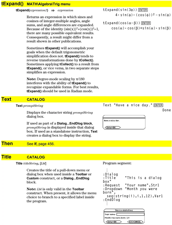
For example, 100_°C converts to 212_°F:
0 100 ←───────────|───────────→ _°C : : ←───────────|───────────→ _°F 32 212
To convert a temperature range, use ΔtmpCnv() instead.
Examples
tmpCnv(100_°c,°f) [ENTER] 212.°F tmpCnv(32_°f,°c) [ENTER] 0.°C tmpCnv(0_°c,°k) [ENTER] 273.15°K tmpCnv(0_°f,°r) [ENTER] 459.67°R
Note: To select temperature units from a menu, press:
TI-89: [2nd] [UNITS]
TI-92 Plus: ◆ [UNITS]
ΔtmpCnv() CATALOG
ΔtmpCnv(expression1_°tempUnit1, °tempUnit2)
⇒ expression°tempUnit2
Converts a temperature range (the difference between two temperature values) specified by expression1 from one unit to another. Valid temperature units are:
- _°C Celsius
- _°F Fahrenheit
- _°K Kelvin
- _°R Rankine
For °, press [2nd] [°].
TI-89: For _, press ◆ [–].
TI-92 Plus: For _, press [2nd] [–].
1_°C and 1_°K have the same magnitude, as do 1_°F and 1_°R. However, 1_°C is 9/5 as large as 1_°F.
Examples
To get Δ, you can press ◆ [□] [↑] [D] (or [2nd] [CHAR] 1 5).
ΔtmpCnv(100_°c,°f) [ENTER] 180.°F ΔtmpCnv(180_°f,°c) [ENTER] 100.°C ΔtmpCnv(100_°c,°k) [ENTER] 100.°K ΔtmpCnv(100_°f,°r) [ENTER] 100.°R ΔtmpCnv(1_°c,°f) [ENTER] 1.8°F
Note: To select temperature units from a menu, press:
TI-89: [2nd] [UNITS]
TI-92 Plus: ◆ [UNITS]
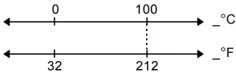
For example, a 100_°C range (from 0_°C to 100_°C) is equivalent to a 180_°F range:
← 100_°C → 0 100 ←───────────|───────────→ _°C : : ←───────────|───────────→ °F 32 212 ← 180°F →
To convert a particular temperature value instead of a range, use tmpCnv().
514 Appendix A: Functions and Instructions
Toolbar CATALOG
Toolbar block EndTBar
Creates a toolbar menu.
block can be either a single statement or a sequence of statements separated with the “:” character. The statements can be either Title or Item.
Items must have labels. A Title must also have a label if it does not have an item.
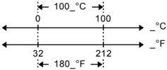
Program segment: ⋮ :Toolbar : Title "Examples" : Item "Trig", t : Item "Calc", c : Item "Stop", Pexit :EndTbar ⋮
Note: When run in a program, this segment creates a menu with three choices that branch to three places in the program.
Trace CATALOG
Trace
Draws a Smart Graph and places the trace cursor on the first defined Y= function at the previously defined cursor position, or at the reset position if regraphing was necessary.
Allows operation of the cursor and most keys when editing coordinate values. Several keys, such as the function keys, APPS, and MODE, are not activated during trace.
Note: Press ENTER to resume operation.
Try CATALOG
Try block1 Else block2 EndTry
Executes block1 unless an error occurs. Program execution transfers to block2 if an error occurs in block1. Variable errnum contains the error number to allow the program to perform error recovery.
block1 and block2 can be either a single statement or a series of statements separated with the “:” character.
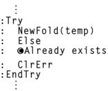
Program segment: ⋮ :Try : NewFold(temp) : Else : @Already exists : ClrErr :EndTry ⋮
Note: See ClrErr and PassErr.
Appendix A: Functions and Instructions 515
TwoVar MATH/Statistics menu
TwoVar list1, list2[, [list3] [, list4, list5]]
Calculates the TwoVar statistics and updates all the system statistics variables.
All the lists must have equal dimensions except for list5.
list1 represents xlist.
list2 represents ylist.
list3 represents frequency.
list4 represents category codes.
list5 represents category include list.
Note: list1 through list4 must be a variable name or c1–c99 (columns in the last data variable shown in the Data/Matrix Editor).
list5 does not have to be a variable name and cannot be c1–c99.
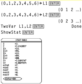
{0,1,2,3,4,5,6}→L1 ENTER
{0 1 2 ...}
{0,2,3,4,3,4,6}→L2 ENTER
{0 2 3 ...}
TwoVar L1,L2 ENTER
Done
ShowStat ENTER
Unarchiv CATALOG
Unarchiv var1 [, var2] [, var3] ...
Moves the specified variables from the user data archive memory to RAM.
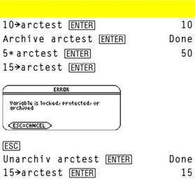
You can access an archived variable the same as you would a variable in RAM. However, you cannot delete, rename, or store to an archived variable because it is locked automatically.
To archive variables, use Archive.
10→arctest ENTER
10
Archive arctest ENTER
Done
5*arctest ENTER
50
15→arctest ENTER
ESC
Unarchiv arctest ENTER
Done
15→arctest ENTER
15
unitV() MATH/Matrix/Vector ops menu
unitV(vector1) ⇒ vector
Returns either a row- or column-unit vector, depending on the form of vector1.
vector1 must be either a single-row matrix or a single-column matrix.
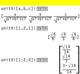
unitV([a,b,c]) ENTER
[ a / √(a²+b²+c²) b / √(a²+b²+c²) c / √(a²+b²+c²) ]
unitV([1,2,1]) ENTER
[ √□/□ √□/□ √□/□ ]
unitV([1;2;3]) ENTER
[ √□□/□□ ]
[ √□□/□ ]
[ 3·√□□/□□ ]
Unlock CATALOG
Unlock var1[, var2][, var3]...
Unlocks the specified variables.
Note: The variables can be locked using the Lock command.
516 Appendix A: Functions and Instructions
variance() MATH/Statistics menu
variance(list[, freqlist]) ⇒ expression
Returns the variance of list.
Each freqlist element counts the number of consecutive occurrences of the corresponding element in list.
Note: list must contain at least two elements.
variance({a,b,c}) ENTER
a² - a·(b+c) + b² - b·c + c²
——————————————
3
variance({1,2,5,-6,3,-2}) ENTER
31/2
variance({1,3,5},{4,6,2}) ENTER
68/33
variance(matrix1[, freqmatrix]) ⇒ matrix
Returns a row vector containing the variance of each column in matrix1.
Each freqmatrix element counts the number of consecutive occurrences of the corresponding element in matrix1.
Note: matrix1 must contain at least two rows.
variance([1,2,5;-3,0,1;.5,.7,3]) ENTER
[4.75 1.03 4]
variance([-1.1,2.2;3.4,5.1;-2.3,4.3],[6,3;2,4;5,1]) ENTER
[3.91731,2.08411]
when() CATALOG
when(condition, trueResult [, falseResult] [, unknownResult]) ⇒ expression
Returns trueResult, falseResult, or unknownResult, depending on whether condition is true, false, or unknown. Returns the input if there are too few arguments to specify the appropriate result.
Omit both falseResult and unknownResult to make an expression defined only in the region where condition is true.
Use an undef falseResult to define an expression that graphs only on an interval.
Omit only the unknownResult to define a two-piece expression.
when(x<0,x+3)|x=5 ENTER
when(x<0,3+x)
ClrGraph ENTER
Graph when(x≥-π and x<0,x+3,undef) ENTER
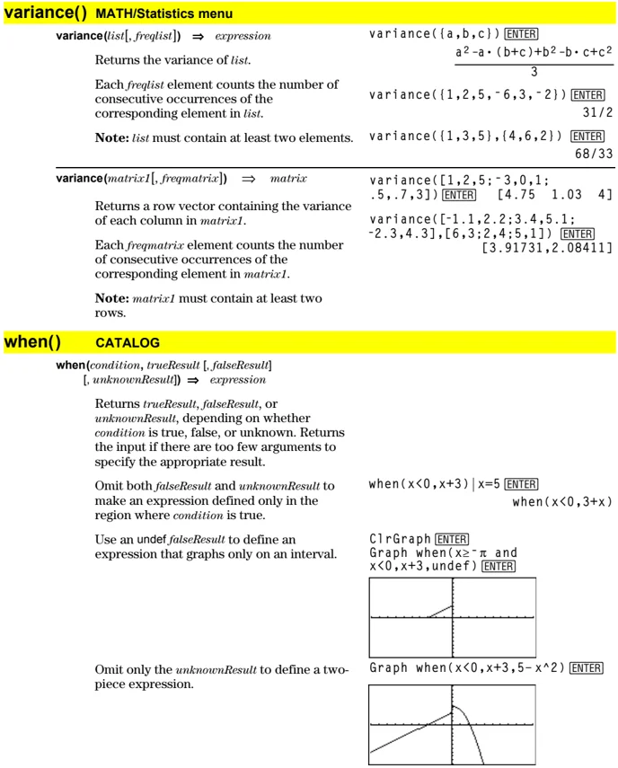
Graph when(x<0,x+3,5-x^2) ENTER
Appendix A: Functions and Instructions 517
Nest when() to define expressions that have more than two pieces.
TI-89: HOME TI-92 Plus: [icon] [HOME]
ClrGraph [ENTER] Done Graph when(x<0,when(x<-π, 4*sin(x),2x+3),5-x^2) [ENTER]
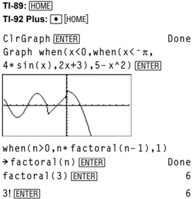
when() is helpful for defining recursive functions.
when(n>0,n*factorial(n-1),1) ⇒factorial(n) [ENTER] Done factorial(3) [ENTER] 6 3! [ENTER] 6
While CATALOG
While condition block EndWhile
Executes the statements in block as long as condition is true.
block can be either a single statement or a sequence of statements separated with the “:” character.
Program segment: ⋮ :1⇒i :0⇒temp :While i<=20 : temp+1/i⇒temp : i+1⇒i :EndWhile :Disp "sum of reciprocals up to 20",temp ⋮
"With" See I, page 538.
xor MATH/Test menu
Boolean expression1 xor Boolean expression2 ⇒ Boolean expression
Returns true if Boolean expression1 is true and Boolean expression2 is false, or vice versa. Returns false if Boolean expression1 and Boolean expression2 are both true or both false. Returns a simplified Boolean expression if either of the original Boolean expressions cannot be resolved to true or false.
Note: See or.
true xor true [ENTER] false (5>3) xor (3>5) [ENTER] true
518 Appendix A: Functions and Instructions
integer1 xor integer2 \Rightarrow integer
Compares two real integers bit-by-bit using an xor operation. Internally, both integers are converted to signed, 32-bit binary numbers. When corresponding bits are compared, the result is 1 if either bit (but not both) is 1; the result is 0 if both bits are 0 or both bits are 1. The returned value represents the bit results, and is displayed according to the Base mode.
You can enter the integers in any number base. For a binary or hexadecimal entry, you must use the 0b or 0h prefix, respectively. Without a prefix, integers are treated as decimal (base 10).
If you enter a decimal integer that is too large for a signed, 32-bit binary form, a symmetric modulo operation is used to bring the value into the appropriate range.
Note: See or.
In Hex base mode: 0h7AC36 xor 0h3D5F [ENTER] 0h79169 \lcorner Important: Zero, not the letter O.
In Bin base mode: 0b100101 xor 0b100 [ENTER] 0b100001
Note: A binary entry can have up to 32 digits (not counting the 0b prefix). A hexadecimal entry can have up to 8 digits.
XorPic CATALOG
XorPic picVar[, row] [, column]
Displays the picture stored in picVar on the current Graph screen.
Uses xor logic for each pixel. Only those pixel positions that are exclusive to either the screen or the picture are turned on. This instruction turns off pixels that are turned on in both images.
picVar must contain a pic data type.
row and column, if included, specify the pixel coordinates for the upper left corner of the picture. Defaults are (0, 0).
zeros() MATH/Algebra menu
zeros(expression, var) \Rightarrow list
Returns a list of candidate real values of var that make expression=0. zeros() does this by computing exp\blacktrianglerightlist(solve(expression=0,var),var).
For some purposes, the result form for zeros() is more convenient than that of solve(). However, the result form of zeros() cannot express implicit solutions, solutions that require inequalities, or solutions that do not involve var.
Note: See also cSolve(), cZeros(), and solve().
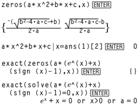
a* x^2+b* x+c ans(1)[2] [ENTER] 0
exact(zeros(a* (e^(x)+x) (sign (x)-1),x)) [ENTER] { }
exact(solve(a* (e^(x)+x) (sign (x)-1)=0,x)) [ENTER] e^x + x = 0 or x > 0 or a = 0
Appendix A: Functions and Instructions 519
zeros(expression1, expression2), {varOrGuess1, varOrGuess2 [, ... ]]) \Rightarrow matrix
Returns candidate real zeros of the simultaneous algebraic expressions, where each varOrGuess specifies an unknown whose value you seek.
Optionally, you can specify an initial guess for a variable. Each varOrGuess must have the form:
variable – or – variable = real or non-real number
For example, x is valid and so is x=3.
If all of the expressions are polynomials and if you do NOT specify any initial guesses, zeros() uses the lexical Gröbner/Buchberger elimination method to attempt to determine all real zeros.
For example, suppose you have a circle of radius r at the origin and another circle of radius r centered where the first circle crosses the positive x-axis. Use zeros() to find the intersections.
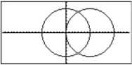
As illustrated by r in the example to the right, simultaneous polynomial expressions can have extra variables that have no values, but represent given numeric values that could be substituted later.
Each row of the resulting matrix represents an alternate zero, with the components ordered the same as the varOrGuess list. To extract a row, index the matrix by [row].
You can also (or instead) include unknowns that do not appear in the expressions. For example, you can include z as an unknown to extend the previous example to two parallel intersecting cylinders of radius r. The cylinder zeros illustrate how families of zeros might contain arbitrary constants in the form @k, where k is an integer suffix from 1 through 255. The suffix resets to 1 when you use ClrHome or [F1] 8:Clear Home.
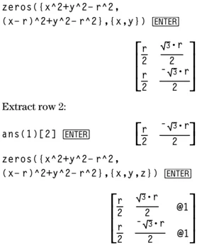
zeros({x^2+y^2-r^2, (x-r)^2+y^2-r^2},{x,y}) ENTER
$$ \begin{bmatrix} \frac{r}{2} & \frac{\sqrt{3}\cdot r}{2} \ \frac{r}{2} & \frac{-\sqrt{3}\cdot r}{2} \end{bmatrix} $$
Extract row 2:
ans(1)(2) ENTER
$$ \begin{bmatrix} \frac{r}{2} & \frac{-\sqrt{3}\cdot r}{2} \end{bmatrix} $$
zeros({x^2+y^2-r^2, (x-r)^2+y^2-r^2},{x,y,z}) ENTER
$$ \begin{bmatrix} \frac{r}{2} & \frac{\sqrt{3}\cdot r}{2} & @1 \ \frac{r}{2} & \frac{-\sqrt{3}\cdot r}{2} & @1 \end{bmatrix} $$
520 Appendix A: Functions and Instructions
For polynomial systems, computation time or memory exhaustion may depend strongly on the order in which you list unknowns. If your initial choice exhausts memory or your patience, try rearranging the variables in the expressions and/or varOrGuess list.
If you do not include any guesses and if any expression is non-polynomial in any variable but all expressions are linear in the unknowns, zeros() uses Gaussian elimination to attempt to determine all real zeros.
If a system is neither polynomial in all of its variables nor linear in its unknowns, zeros() determines at most one zero using an approximate iterative method. To do so, the number of unknowns must equal the number of expressions, and all other variables in the expressions must simplify to numbers.
Each unknown starts at its guessed value if there is one; otherwise, it starts at 0.0.
Use guesses to seek additional zeros one by one. For convergence, a guess may have to be rather close to a zero.
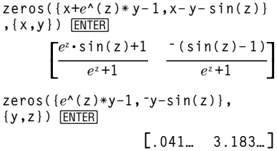
zeros({x+e^(z)*y-1,x-y-sin(z)} ,{x,y}) ENTER
$$ \left[ \frac{e^z \cdot \sin(z)+1}{e^z+1} \quad \frac{-(\sin(z)-1)}{e^z+1} \right] $$
zeros({e^(z)*y-1,-y-sin(z)}, {y,z}) ENTER
[.041... 3.183...]
zeros({e^(z)*y-1,-y-sin(z)}, {y,z=2π}) ENTER
[.001... 6.281...]
ZoomBox CATALOG
ZoomBox
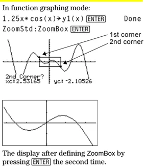
Displays the Graph screen, lets you draw a box that defines a new viewing window, and updates the window.
In function graphing mode:
1.25x*\cos(x) \rightarrow y1(x) ENTER Done
ZoomStd:ZoomBox ENTER
The display after defining ZoomBox by pressing ENTER the second time.
Appendix A: Functions and Instructions 521
ZoomData CATALOG
ZoomData
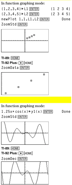
Adjusts the window settings based on the currently defined plots (and data) so that all statistical data points will be sampled, and displays the Graph screen.
Note: Does not adjust ymin and ymax for histograms.
In function graphing mode: (1,2,3,4) \rightarrow L1 [ENTER] {1 2 3 4} (2,3,4,5) \rightarrow L2 [ENTER] {2 3 4 5} newPlot 1,1,L1,L2 [ENTER] Done ZoomStd [ENTER]
TI-89: [HOME] TI-92 Plus: [HOME] ZoomData [ENTER]
ZoomDec CATALOG
ZoomDec
Adjusts the viewing window so that \Delta x and \Delta y = 0.1 and displays the Graph screen with the origin centered on the screen.
In function graphing mode: 1.25x*cos(x) \rightarrow y1(x) [ENTER] Done ZoomStd [ENTER]
TI-89: [HOME] TI-92 Plus: [HOME] ZoomDec [ENTER]
522 Appendix A: Functions and Instructions
ZoomFit CATALOG
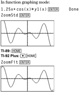
ZoomFit Displays the Graph screen, and calculates the necessary window dimensions for the dependent variables to view all the picture for the current independent variable settings.
In function graphing mode: 1.25x*cos(x)→y1(x) [ENTER] Done ZoomStd [ENTER]
TI-89: [HOME] TI-92 Plus: [●][HOME] ZoomFit [ENTER]
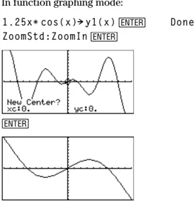
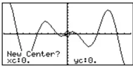
ZoomIn CATALOG
ZoomIn Displays the Graph screen, lets you set a center point for a zoom in, and updates the viewing window.
The magnitude of the zoom is dependent on the Zoom factors xFact and yFact. In 3D Graph mode, the magnitude is dependent on xFact, yFact, and zFact.
In function graphing mode: 1.25x*cos(x)→y1(x) [ENTER] Done ZoomStd:ZoomIn [ENTER]
New Center? xc=0. yc=0. [ENTER]
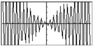
ZoomInt CATALOG
ZoomInt Displays the Graph screen, lets you set a center point for the zoom, and adjusts the window settings so that each pixel is an integer in all directions.
In function graphing mode: 1.25x*cos(x)→y1(x) [ENTER] Done ZoomStd:ZoomInt [ENTER]
New Center? xc=0. yc=0. [ENTER]
Appendix A: Functions and Instructions 523
ZoomOut CATALOG
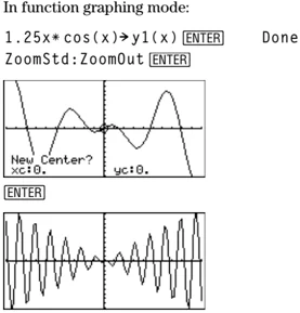
ZoomOut
Displays the Graph screen, lets you set a center point for a zoom out, and updates the viewing window.
The magnitude of the zoom is dependent on the Zoom factors xFact and yFact. In 3D Graph mode, the magnitude is dependent on xFact, yFact, and zFact.
In function graphing mode:
1.25x*cos(x)→y1(x) [ENTER] Done ZoomStd:ZoomOut [ENTER]
ZoomPrev CATALOG
ZoomPrev
Displays the Graph screen, and updates the viewing window with the settings in use before the last zoom.
ZoomRcl CATALOG
ZoomRcl
Displays the Graph screen, and updates the viewing window using the settings stored with the ZoomSto instruction.
ZoomSqr CATALOG
ZoomSqr
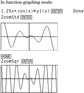
Displays the Graph screen, adjusts the x or y window settings so that each pixel represents an equal width and height in the coordinate system, and updates the viewing window.
In 3D Graph mode, ZoomSqr lengthens the shortest two axes to be the same as the longest axis.
In function graphing mode:
1.25x*cos(x)→y1(x) [ENTER] Done ZoomStd [ENTER]
524 Appendix A: Functions and Instructions
ZoomStd CATALOG
ZoomStd
Sets the window variables to the following standard values, and then updates the viewing window.
Function graphing: x: [⁻10, 10, 1], y: [⁻10, 10, 1] and xres=2
Parametric graphing: t: [0, 2π, π/24], x: [⁻10, 10, 1], y:[⁻10, 10, 1]
Polar graphing: θ: [0, 2π, π/24], x: [⁻10, 10, 1], y: [⁻10, 10, 1]
Sequence graphing: nmin=1, nmax=10, plotStrt=1, plotStep=1, x: [⁻10, 10, 1], y: [⁻10, 10, 1]
3D graphing: eyeθ°=20, eyeφ°=70, eyeψ°=0 x: [⁻10, 10, 14], y: [⁻10, 10, 14], z: [⁻10, 10], ncontour=5
Differential equations graphing: t: [0, 10, .1, 0], x: [⁻1, 10, 1], y: [⁻10, 10, 1], ncurves=0, Estep=1, difftol=.001, fldres=14, dtime=0
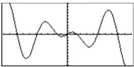
In function graphing mode: 1.25x*cos(x)►y1(x) ENTER Done ZoomStd ENTER
ZoomSto CATALOG
ZoomSto
Stores the current Window settings in the Zoom memory. You can use ZoomRcl to restore the settings.
ZoomTrig CATALOG
ZoomTrig
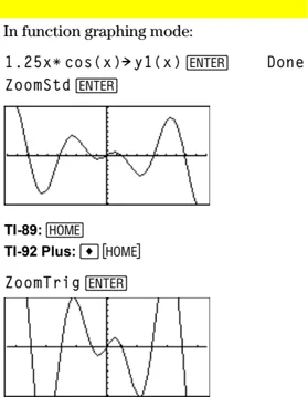
Displays the Graph screen, sets \Deltax to \pi/24, and xsel to \pi/2, centers the origin, sets the y settings to [⁻4, 4, .5], and updates the viewing window.
In function graphing mode: 1.25x*cos(x)►y1(x) ENTER Done ZoomStd ENTER
TI-89: HOME TI-92 Plus: HOME
ZoomTrig ENTER
Appendix A: Functions and Instructions 525
- (add) [+] key
expression1 + expression2 ⇒ expression Returns the sum of expression1 and expression2.
56 ENTER ans(1)+4 ENTER ans(1)+4 ENTER ans(1)+4 ENTER ans(1)+4 ENTER
56 60 64 68 72
list1 + list2 ⇒ list matrix1 + matrix2 ⇒ matrix Returns a list (or matrix) containing the sums of corresponding elements in list1 and list2 (or matrix1 and matrix2). Dimensions of the arguments must be equal.
{22,π,π/2}→L1 ENTER {10,5,π/2}→L2 ENTER L1+L2 ENTER ans(1)+{π,-5,-π} ENTER [a,b;c,d]+[1,0;0,1] ENTER
{22 π π/2} {10 5 π/2} {32 π+5 π} {π+32 π 0} [ a+1 b ] [ c d+1 ]
expression + list1 ⇒ list list1 + expression ⇒ list Returns a list containing the sums of expression and each element in list1.
15+{10,15,20} ENTER {10,15,20}+15 ENTER
{25 30 35} {25 30 35}
expression + matrix1 ⇒ matrix matrix1 + expression ⇒ matrix Returns a matrix with expression added to each element on the diagonal of matrix1. matrix1 must be square. Note: Use .+ (dot plus) to add an expression to each element.
20+[1,2;3,4] ENTER
[21 2] [3 24]
− (subtract) [−] key
expression1 - expression2 ⇒ expression Returns expression1 minus expression2.
6−2 ENTER π−π/6 ENTER
4 5·π — 6
list1 - list2 ⇒ list matrix1 - matrix2 ⇒ matrix Subtracts each element in list2 (or matrix2) from the corresponding element in list1 (or matrix1), and returns the results. Dimensions of the arguments must be equal.
{22,π,π/2}−{10,5,π/2} ENTER [3,4]−[1,2] ENTER
{12 π−5 0} [2 2]
expression - list1 ⇒ list list1 - expression ⇒ list Subtracts each list1 element from expression or subtracts expression from each list1 element, and returns a list of the results.
15−{10,15,20} ENTER {10,15,20}−15 ENTER
{5 0 -5} {-5 0 5}
526 Appendix A: Functions and Instructions
expression - matrix1 ⇒ matrix matrix1 - expression ⇒ matrix
20 - [1,2;3,4] ENTER 19 -2 [ -3 16]
expression - matrix1 returns a matrix of expression times the identity matrix minus matrix1. matrix1 must be square.
matrix1 - expression returns a matrix of expression times the identity matrix subtracted from matrix1. matrix1 must be square.
Note: Use .- (dot minus) to subtract an expression from each element.
* (multiply) × key
expression1 * expression2 ⇒ expression
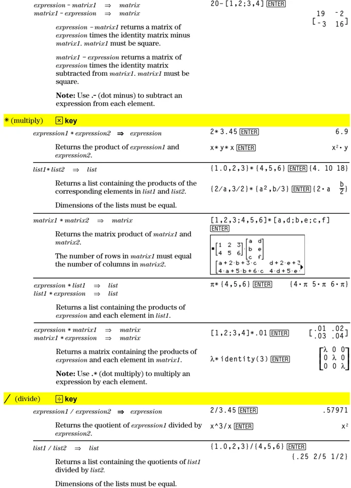
2 * 3.45 ENTER 6.9
x * y * x ENTER x² · y
Returns the product of expression1 and expression2.
list1 * list2 ⇒ list
{1.0,2,3} * {4,5,6} ENTER {4. 10 18}
{2/a,3/2} * {a²,b/3} ENTER {2·a b/2}
Returns a list containing the products of the corresponding elements in list1 and list2.
Dimensions of the lists must be equal.
matrix1 * matrix2 ⇒ matrix
[1,2,3;4,5,6] * [a,d;b,e;c,f] ENTER [1 2 3] [a d] [4 5 6] [b e] [c f] [a+2·b+3·c d+2·e+3·f] [4·a+5·b+6·c 4·d+5·e·f]
Returns the matrix product of matrix1 and matrix2.
The number of rows in matrix1 must equal the number of columns in matrix2.
expression * list1 ⇒ list list1 * expression ⇒ list
π * {4,5,6} ENTER {4·π 5·π 6·π}
Returns a list containing the products of expression and each element in list1.
expression * matrix1 ⇒ matrix matrix1 * expression ⇒ matrix
[1,2;3,4] * .01 ENTER [.01 .02] [.03 .04]
λ * identity(3) ENTER [λ 0 0] [0 λ 0] [0 0 λ]
Returns a matrix containing the products of expression and each element in matrix1.
Note: Use .* (dot multiply) to multiply an expression by each element.
/ (divide) ÷ key
expression1 / expression2 ⇒ expression
2 / 3.45 ENTER
- 57971
x^3 / x ENTER x²
Returns the quotient of expression1 divided by expression2.
list1 / list2 ⇒ list
{1.0,2,3} / {4,5,6} ENTER {.25 2/5 1/2}
Returns a list containing the quotients of list1 divided by list2.
Dimensions of the lists must be equal.
Appendix A: Functions and Instructions 527
expression / list1 ⇒ list list1 / expression ⇒ list
Returns a list containing the quotients of expression divided by list1 or list1 divided by expression.
a / { 3 , a , √( a ) } [ENTER] { a/3 1 √a }
{ a , b , c } / ( a * b * c ) [ENTER] { 1/b \cdot c 1/a \cdot c 1/a \cdot b }
matrix1 / expression ⇒ matrix
Returns a matrix containing the quotients of matrix1 / expression.
[ a , b , c ] / ( a * b * c ) [ENTER] [ 1/b \cdot c 1/a \cdot c 1/a \cdot b ]
Note: Use ./ (dot divide) to divide an expression by each element.
⁻ (negate) [(-)] key and MATH/Base menu
- expression1 ⇒ expression
- list1 ⇒ list
- matrix1 ⇒ matrix
Returns the negation of the argument.
For a list or matrix, returns all the elements negated.
If expression1 is a binary or hexadecimal integer, the negation gives the two’s complement.
-
2.43 [ENTER] -2.43
-
{ -1 , 0.4 , 1.2 E 19 } [ENTER] { 1 -.4 -1.2E19 }
-
a * - b [ENTER] a · b
In Bin base mode:
0b100101 ▶ dec [ENTER] 37
└─ Important: Zero, not the letter O.
- 0b100101 [ENTER] 0b1111111111111111111111111011011
ans(1) ▶ dec [ENTER] -37
Note: To type ▶, press [2nd] [▶].
% (percent) CHAR/Punctuation menu
expression1 % ⇒ expression list1 % ⇒ list matrix1 % ⇒ matrix
Returns argument/100.
For a list or matrix, returns a list or matrix with each element divided by 100.
13% ◆ [ENTER] .13
{ 1 , 10 , 100 } % ◆ [ENTER] { .01 .1 1. }
528 Appendix A: Functions and Instructions