part() CATALOG
part(expression1[,nonNegativeInteger])
This advanced programming function lets you identify and extract all of the sub-expressions in the simplified result of expression1.
For example, if expression1 simplifies to cos(π* x+3):
- The cos() function has one argument: (π* x+3).
- The sum of (π* x+3) has two operands: π* x and 3.
- The number 3 has no arguments or operands.
- The product π* x has two operands: π and x.
- The variable x and the symbolic constant π have no arguments or operands.
If x has a numeric value and you press [▶] [ENTER], the numeric value of π* x is calculated, the result is added to 3, and then the cosine is calculated. cos() is the top-level operator because it is applied last.
\begin{tabular}{p{0.55\textwidth} p{0.4\textwidth}} part(expression1) \Rightarrow number & part(cos(\pix+3)) \texttt{[ENTER]} 1 \ Simplifies expression1 and returns the number of top-level arguments or operands. This returns 0 if expression1 is a number, variable, or symbolic constant such as \pi, $e$, \boldsymboli, or \infty. & \textbf{Note:} cos(\pix+3) has one argument. \ part(expression1, 0) \Rightarrow string & part(cos(\pix+3),0) \texttt{[ENTER]} "cos" \ Simplifies expression1 and returns a string that contains the top-level function name or operator. This returns string(expression1) if expression1 is a number, variable, or symbolic constant such as \pi, $e$, \boldsymboli, or \infty. & \ part(expression1, n) \Rightarrow expression & part(cos(\pix+3),1) \texttt{[ENTER]} 3+\pi\cdotx \ Simplifies expression1 and returns the $n^{th}$ argument or operand, where $n$ is $> 0$ and \leq the number of top-level arguments or operands returned by part(expression1). Otherwise, an error is returned. & \textbf{Note:} Simplification changed the order of the argument. \ \end{tabular}
Appendix A: Functions and Instructions 477
By combining the variations of part(), you can extract all of the sub-expressions in the simplified result of expression1. As shown in the example to the right, you can store an argument or operand and then use part() to extract further sub-expressions.
Note: When using part(), do not rely on any particular order in sums and products.
Expressions such as (x+y+z) and (x-y-z) are represented internally as (x+y)+z and (x-y)-z. This affects the values returned for the first and second argument. There are technical reasons why part(x+y+z,1) returns y+x instead of x+y.
Similarly, xyz is represented internally as (xy)z. Again, there are technical reasons why the first argument is returned as yx instead of xy.
When you extract sub-expressions from a matrix, remember that matrices are stored as lists of lists, as illustrated in the example to the right.
\begin{tabular}{ll} part(cos(\pix+3)) \textsc{enter} & 1 \ part(cos(\pix+3),0) \textsc{enter} & "cos" \ part(cos(\pix+3),1)\rightarrowtemp \textsc{enter} & 3+\pi\cdotx \ temp \textsc{enter} & \pi\cdotx+3 \ part(temp,0) \textsc{enter} & "+" \ part(temp) \textsc{enter} & 2 \ part(temp,2) \textsc{enter} & 3 \ part(temp,1)\rightarrowtemp \textsc{enter} & \pi\cdotx \ part(temp,0) \textsc{enter} & "" \ part(temp) \textsc{enter} & 2 \ part(temp,1) \textsc{enter} & \pi \ part(temp,2) \textsc{enter} & x \ part(x+y+z) \textsc{enter} & 2 \ part(x+y+z,2) \textsc{enter} & z \ part(x+y+z,1) \textsc{enter} & y+x \ part(xyz) \textsc{enter} & 2 \ part(xyz,2) \textsc{enter} & z \ part(xyz,1) \textsc{enter} & y*x \ part([a,b,c;x,y,z],0) \textsc{enter} & "{" \ part([a,b,c;x,y,z]) \textsc{enter} & 2 \ part([a,b,c;x,y,z],2)\rightarrowtemp & \ \textsc{enter} & {x \quad y \quad z} \ part(temp,0) \textsc{enter} & "{" \ part(temp) \textsc{enter} & 3 \ part(temp,3) \textsc{enter} & z \ delVar temp \textsc{enter} & Done \ \end{tabular}
478 Appendix A: Functions and Instructions
The example Program Editor function to the right uses getType() and part() to partially implement symbolic differentiation. Studying and completing this function can help teach you how to differentiate manually. You could even include functions that the TI-89 / TI-92 Plus cannot differentiate, such as Bessel functions.
\begin{tabular}{p{0.48\textwidth} p{0.48\textwidth}} : d(y,x) & \ : Func & \ : Local f & \ : If getType(y)="VAR" & \ : \quad Return when(y=x,1,0,0) & \ : If part(y)=0 & \ : \quad Return 0 ● y=π,∞,i,numbers & \ : part(y,0)→f & \ : If f="-" ● if negate & \ : \quad Return -d(part(y,1),x) & \ : If f="-" ● if minus & \ : \quad Return d(part(y,1),x) & \ : \quad \quad -d(part(y,2),x) & \ : If f="+" & \ : \quad Return d(part(y,1),x) & \ : \quad \quad +d(part(y,2),x) & \ : If f="*" & \ : \quad Return & \ : \quad part(y,1)*d(part(y,2),x) & \ : \quad \quad +part(y,2)*d(part(y,1),x) & \ : If f="{" & \ : \quad Return seq(d(part(y,k),x), & \ : \quad \quad k,1,part(y)) & \ : Return undef & \ : EndFunc & \ & \ \textbf{PassErr} \quad CATALOG & See ClrErr program listing example. \ PassErr & Passes an error to the next level. \ & If "errornum" is zero, PassErr does not do anything. \ & The Else clause in the program should use ClrErr or PassErr. If the error is to be processed or ignored, use ClrErr. If what to do with the error is not known, use PassErr to send it to the next error handler. (See also ClrErr.) \ & \ \textbf{Pause} \quad CATALOG & Program segment: \ Pause [expression] & : \ & : ClrIO \ & : DelVar temp \ & : 1→temp[1] \ & : 1→temp[2] \ & : Disp temp[2] \ & : ● Guess the Pattern \ & : For i,3,20 \ & : \quad temp[i-2]+temp[i-1]→temp[i] \ & : \quad Disp temp[i] \ & : \quad Disp temp,"Can you guess the next","number?" \ & : Pause \ & : EndFor \ & : \ Suspends program execution. If you include expression, displays expression on the Program I/O screen. & \ expression can include conversion operations such as \blacktrianglerightDD and \blacktrianglerightRect. You can also use the \blacktriangleright operator to perform unit and number base conversions. & \ If the result of expression is too big to fit on a single screen, you can use the cursor pad to scroll the display. & \ Program execution resumes when you press ENTER. & \ \end{tabular}
Appendix A: Functions and Instructions 479
PlotsOff CATALOG
PlotsOff [1] [, 2] [, 3] ... [, 9] Turns off the specified plots for graphing. When in 2-graph mode, only affects the active graph. If no parameters, then turns off all plots.
PlotsOff 1,2,5 ENTER Done PlotsOff ENTER Done
PlotsOn CATALOG
PlotsOn [1] [, 2] [, 3] ... [, 9] Turns on the specified plots for graphing. When in 2-graph mode, only affects the active graph. If you do not include any arguments, turns on all plots.
PlotsOn 2,4,5 ENTER Done PlotsOn ENTER Done
▶Polar MATH/Matrix/Vector ops menu
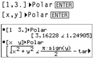
vector▶Polar Displays vector in polar form [r ∠θ]. The vector must be of dimension 2 and can be a row or a column.
Note: ▶Polar is a display-format instruction, not a conversion function. You can use it only at the end of an entry line, and it does not update ans.
Note: See also ▶Rect.
[1,3.]▶Polar ENTER [x,y]▶Polar ENTER
complexValue▶Polar Displays complexVector in polar form.
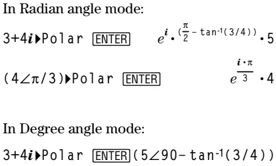
- Degree angle mode returns (r∠θ).
- Radian angle mode returns re^i\theta.
complexValue can have any complex form. However, an re^i\theta entry causes an error in Degree angle mode.
Note: You must use the parentheses for an (r∠θ) polar entry.
In Radian angle mode: $3+4i$▶Polar ENTER e^i \cdot (\pi/2 - \tan^-1(3/4)) \cdot .5 (4\angle3)▶Polar ENTER i \cdot \pi/e^3 \cdot .4
In Degree angle mode: $3+4i$▶Polar ENTER (5\angle90-\tan^-1(3/4))
polyEval() MATH/List menu
polyEval(list1, expression1) \Rightarrow expression polyEval(list1, list2) \Rightarrow expression
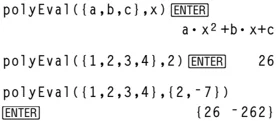
Interprets the first argument as the coefficient of a descending-degree polynomial, and returns the polynomial evaluated for the value of the second argument.
polyEval({a,b,c},x) ENTER a \cdot x^2 + b \cdot x + c polyEval({1,2,3,4},2) ENTER 26 polyEval({1,2,3,4},{2,-7}) ENTER {26 -262}
480 Appendix A: Functions and Instructions

PopUp CATALOG
PopUp itemList, var
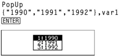
Displays a pop-up menu containing the character strings from itemList, waits for you to select an item, and stores the number of your selection in var.
The elements of itemList must be character strings: {item1String, item2String, item3String, ...}
If var already exists and has a valid item number, that item is displayed as the default choice.
itemList must contain at least one choice.
PopUp {"□□□□","□□□□","□□□□"},var1
ENTER
PowerReg MATH/Statistics/Regressions menu
PowerReg list1, list2[, [list3] [, list4, list5]]
Calculates the power regression and updates all the system statistics variables.
All the lists must have equal dimensions except for list5.
list1 represents xlist.
list2 represents ylist.
list3 represents frequency.
list4 represents category codes.
list5 represents category include list.
Note: list1 through list4 must be a variable name or c1–c99 (columns in the last data variable shown in the Data/Matrix Editor). list5 does not have to be a variable name and cannot be c1–c99.
In function graphing mode:
{1,2,3,4,5,6,7}→L1 ENTER
{1 2 3 ...}
{1,2,3,4,3,4,6}→L2 ENTER
{1 2 3 ...}
PowerReg L1,L2 ENTER Done
ShowStat ENTER
 ENTER
Regeq(x)→y1(x) ENTER Done
NewPlot 1,1,L1,L2 ENTER Done
♦ [GRAPH]
Prgm CATALOG
Prgm
:
EndPrgm
Required instruction that identifies the beginning of a program. Last line of program must be EndPrgm.
Program segment:
:prgmname()
:Prgm
:
:EndPrgm
Appendix A: Functions and Instructions 481
product() MATH/List menu
product(list[, start[, end]]) ⇒ expression
Returns the product of the elements contained in list. Start and end are optional. They specify a range of elements.
product({1,2,3,4}) ENTER 24
product({2,x,y}) ENTER 2·x·y
product({4,5,8,9},2,3) ENTER 40
product(matrixI[, start[, end]]) ⇒ matrix
Returns a row vector containing the products of the elements in the columns of matrixI. Start and end are optional. They specify a range of rows.
product([1,2,3;4,5,6;7,8,9]) ENTER [28 80 162]
product([1,2,3;4,5,6;7,8,9], 1,2) ENTER [4,10,18]
Prompt CATALOG
Prompt var1[, var2] [, var3] ...
Displays a prompt on the Program I/O screen for each variable in the argument list, using the prompt var1?. Stores the entered expression in the corresponding variable.
Prompt must have at least one argument.
Program segment:
: Prompt A,B,C : EndPrgm
propFrac() MATH/Algebra menu
propFrac(expressionI[, var]) ⇒ expression
propFrac(rational_number) returns rational_number as the sum of an integer and a fraction having the same sign and a greater denominator magnitude than numerator magnitude.
propFrac(rational_expression,var) returns the sum of proper ratios and a polynomial with respect to var. The degree of var in the denominator exceeds the degree of var in the numerator in each proper ratio. Similar powers of var are collected. The terms and their factors are sorted with var as the main variable.
If var is omitted, a proper fraction expansion is done with respect to the most main variable. The coefficients of the polynomial part are then made proper with respect to their most main variable first and so on.
For rational expressions, propFrac() is a faster but less extreme alternative to expand().
propFrac(4/3) ENTER 1 + 1/3
propFrac(-4/3) ENTER -1-1/3
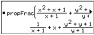
propFrac((x^2+x+1)/(x+1)+(y^2+y+1)/(y+1),x) ENTER
■ propFrac( (x²+x+1)/(x+1) + (y²+y+1)/(y+1) ) 1/(x+1) + x + (y²+y+1)/(y+1)
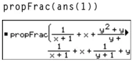
propFrac(ans(1))
■ propFrac( 1/(x+1) + x + (y²+y+1)/(y+1) ) 1/(x+1) + x + 1/(y+1) + y
PtChg CATALOG
PtChg x, y
PtChg xList, yList
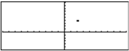
Displays the Graph screen and reverses the screen pixel nearest to window coordinates (x, y).
Note: PtChg through PtText show continuing similar examples.
PtChg 2,4 ENTER
482 Appendix A: Functions and Instructions
PtOff CATALOG
PtOff x, y PtOff xList, yList
Displays the Graph screen and turns off the screen pixel nearest to window coordinates (x, y).
PtOff 2,4 [ENTER]
PtOn CATALOG
PtOn x, y PtOn xList, yList
Displays the Graph screen and turns on the screen pixel nearest to window coordinates (x, y).
PtOn 3,5 [ENTER]
ptTest() CATALOG
ptTest (x, y) \Rightarrow Boolean constant expression ptTest (xList, yList) \Rightarrow Boolean constant expression
Returns true or false. Returns true only if the screen pixel nearest to window coordinates (x, y) is on.
ptTest(3,5) [ENTER] true
PtText CATALOG
PtText string, x, y
Displays the Graph screen and places the character string string on the screen at the pixel nearest the specified (x, y) window coordinates.
string is positioned with the upper-left corner of its first character at the coordinates.
PtText "sample",3,5 [ENTER]
PxlChg CATALOG
PxlChg row, col PxlChg rowList, colList
Displays the Graph screen and reverses the pixel at pixel coordinates (row, col).
Note: Regraphing erases all drawn items.
PxlChg 2,4 [ENTER]
PxlCrcl CATALOG
PxlCrcl row, col, r [, drawMode]
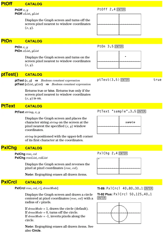
Displays the Graph screen and draws a circle centered at pixel coordinates (row, col) with a radius of r pixels.
If drawMode = 1, draws the circle (default). If drawMode = 0, turns off the circle. If drawMode = -1, inverts pixels along the circle.
Note: Regraphing erases all drawn items. See also Circle.
TI-89: PxlCrcl 40,80,30,1 [ENTER] TI-92 Plus: PxlCrcl 50,125,40,1 [ENTER]
Appendix A: Functions and Instructions 483
PxlHorz CATALOG
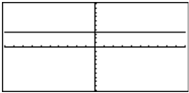
PxlHorz row [, drawMode]
Displays the Graph screen and draws a horizontal line at pixel position row.
If drawMode = 1, draws the line (default). If drawMode = 0, turns off the line. If drawMode = -1, turns a line that is on to off or off to on (inverts pixels along the line).
Note: Regraphing erases all drawn items. See also LineHorz.
PxlHorz 25,1 [ENTER]
PxlLine CATALOG
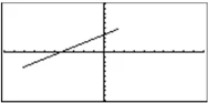
PxlLine rowStart, colStart, rowEnd, colEnd [, drawMode]
Displays the Graph screen and draws a line between pixel coordinates (rowStart, colStart) and (rowEnd, colEnd), including both endpoints.
If drawMode = 1, draws the line (default). If drawMode = 0, turns off the line. If drawMode = -1, turns a line that is on to off or off to on (inverts pixels along the line).
Note: Regraphing erases all drawn items. See also Line.
TI-89: PxlLine 50,15,20,90,1 [ENTER] TI-92 Plus: PxlLine 80,20,30,150,1 [ENTER]
PxlOff CATALOG
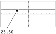
PxlOff row, col PxlOff rowList, colList
Displays the Graph screen and turns off the pixel at pixel coordinates (row, col).
Note: Regraphing erases all drawn items.
PxlHorz 25,1 [ENTER] PxlOff 25,50 [ENTER]
25,50
PxlOn CATALOG
PxlOn row, col PxlOn rowList, colList
Displays the Graph screen and turns on the pixel at pixel coordinates (row, col).
Note: Regraphing erases all drawn items.
PxlOn 25,50 [ENTER]
pxlTest() CATALOG
pxlTest (row, col) \Rightarrow Boolean expression pxlTest (rowList, colList) \Rightarrow Boolean expression
Returns true if the pixel at pixel coordinates (row, col) is on. Returns false if the pixel is off.
Note: Regraphing erases all drawn items.
PxlOn 25,50 [ENTER] TI-89: [HOME] TI-92 Plus: [HOME] PxlTest(25,50) [ENTER] true PxlOff 25,50 [ENTER] TI-89: [HOME] TI-92 Plus: [HOME] PxlTest(25,50) [ENTER] false
484 Appendix A: Functions and Instructions
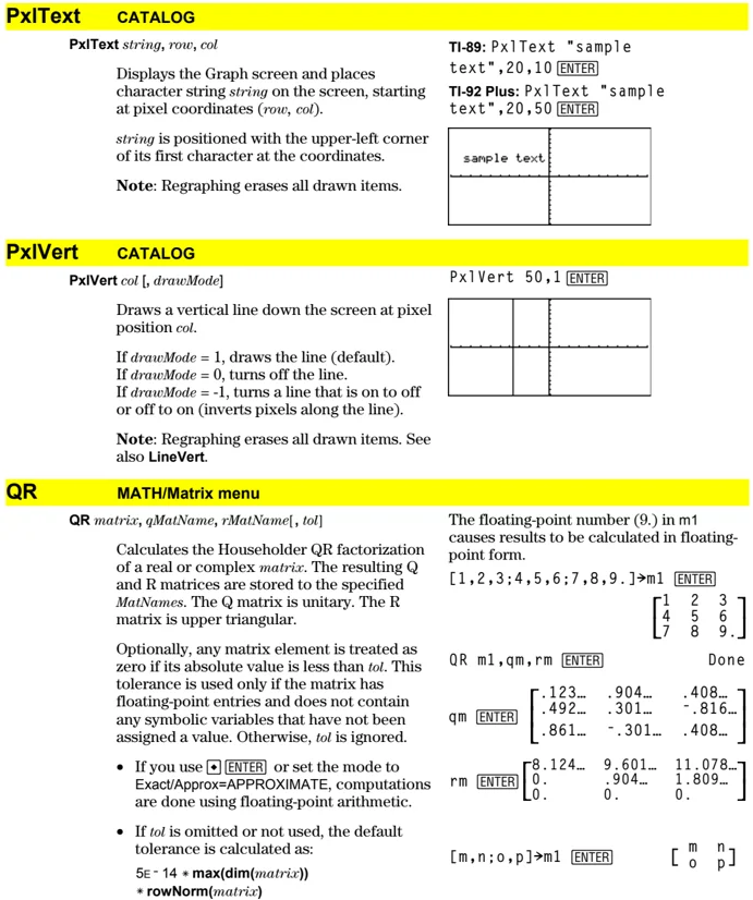
PxlText CATALOG
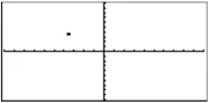
PxlText string, row, col
Displays the Graph screen and places character string string on the screen, starting at pixel coordinates (row, col).
string is positioned with the upper-left corner of its first character at the coordinates.
Note: Regraphing erases all drawn items.
TI-89: PxlText "sample text",20,10 ENTER TI-92 Plus: PxlText "sample text",20,50 ENTER
PxlVert CATALOG
PxlVert col [, drawMode]
Draws a vertical line down the screen at pixel position col.
If drawMode = 1, draws the line (default). If drawMode = 0, turns off the line. If drawMode = -1, turns a line that is on to off or off to on (inverts pixels along the line).
Note: Regraphing erases all drawn items. See also LineVert.
PxlVert 50,1 ENTER
QR MATH/Matrix menu
QR matrix, qMatName, rMatName[, tol]
Calculates the Householder QR factorization of a real or complex matrix. The resulting Q and R matrices are stored to the specified MatNames. The Q matrix is unitary. The R matrix is upper triangular.
Optionally, any matrix element is treated as zero if its absolute value is less than tol. This tolerance is used only if the matrix has floating-point entries and does not contain any symbolic variables that have not been assigned a value. Otherwise, tol is ignored.
- If you use [■] ENTER or set the mode to Exact/Approx=APPROXIMATE, computations are done using floating-point arithmetic.
- If tol is omitted or not used, the default tolerance is calculated as: 5E-14 * max(dim(matrix)) *rowNorm(matrix)
The floating-point number (9.) in m1 causes results to be calculated in floating-point form.
[1,2,3;4,5,6;7,8,9.]→m1 ENTER
$$ \begin{bmatrix} 1 & 2 & 3 \ 4 & 5 & 6 \ 7 & 8 & 9. \end{bmatrix} $$
QR m1,qm,rm ENTER Done
qm ENTER
$$ \begin{bmatrix} .123... & .904... & .408... \ .492... & .301... & -.816... \ .861... & -.301... & .408... \end{bmatrix} $$
rm ENTER
$$ \begin{bmatrix} 8.124... & 9.601... & 11.078... \ 0. & .904... & 1.809... \ 0. & 0. & 0. \end{bmatrix} $$
[m,n;o,p]→m1 ENTER
$$ \begin{bmatrix} m & n \ o & p \end{bmatrix} $$
Appendix A: Functions and Instructions 485
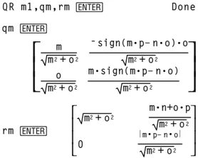
The QR factorization is computed numerically using Householder transformations. The symbolic solution is computed using Gram-Schmidt. The columns in qMatName are the orthonormal basis vectors that span the space defined by matrix.
QR m1, qm, rm \boxedENTER Done
qm \boxedENTER $$ \begin{bmatrix} \frac{m}{\sqrt{m^2+o^2}} & \frac{-\text{sign}(m \cdot p - n \cdot o) \cdot o}{\sqrt{m^2+o^2}} \ \frac{o}{\sqrt{m^2+o^2}} & \frac{m \cdot \text{sign}(m \cdot p - n \cdot o)}{\sqrt{m^2+o^2}} \end{bmatrix} $$
rm \boxedENTER $ \beginbmatrix \sqrtm^2+o^2 & \fracm \cdot n + o \cdot p\sqrtm^2+o^2 \ 0 & \frac|m \cdot p - n \cdot o|\sqrtm^2+o^2 \endbmatrix $
QuadReg MATH/Statistics/Regressions menu
QuadReg list1, list2[, [list3] [, list4, list5]]
Calculates the quadratic polynomial regression and updates the system statistics variables.
All the lists must have equal dimensions except for list5.
list1 represents xlist. list2 represents ylist. list3 represents frequency. list4 represents category codes. list5 represents category include list.
Note: list1 through list4 must be a variable name or c1–c99. (columns in the last data variable shown in the Data/Matrix Editor). list5 does not have to be a variable name and cannot be c1–c99.
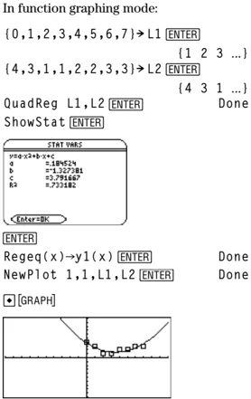
In function graphing mode:
(0,1,2,3,4,5,6,7) \rightarrow L1 \boxedENTER {1 2 3 ...} (4,3,1,1,2,2,3,3) \rightarrow L2 \boxedENTER {4 3 1 ...}
QuadReg L1,L2 \boxedENTER Done ShowStat \boxedENTER
\boxedENTER Regeq(x) \rightarrow y1(x) \boxedENTER Done NewPlot 1,1,L1,L2 \boxedENTER Done
\boxed\blacksquare [GRAPH]
486 Appendix A: Functions and Instructions
QuartReg MATH/Statistics/Regressions menu
QuartReg list1, list2[, [list3] [, list4, list5]]
Calculates the quartic polynomial regression and updates the system statistics variables.
All the lists must have equal dimensions except for list5.
list1 represents xlist. list2 represents ylist. list3 represents frequency. list4 represents category codes. list5 represents category include list.
Note: list1 through list4 must be a variable name or c1–c99 (columns in the last data variable shown in the Data/Matrix Editor). list5 does not have to be a variable name and cannot be c1–c99.
In function graphing mode:
{-2,-1,0,1,2,3,4,5,6}►L1 ENTER
{-2 -1 0 ...}
{4,3,1,2,4,2,1,4,6}►L2 ENTER
{4 3 1 ...}
QuartReg L1,L2 ENTER Done
ShowStat ENTER
 ENTER
Regeq(x)→y1(x) ENTER Done
NewPlot 1,1,L1,L2 ENTER Done
▶ [GRAPH]
R▶Pθ() MATH/Angle menu
R▶Pθ (xExpression, yExpression) ⇒ expression R▶Pθ (xList, yList) ⇒ list R▶Pθ (xMatrix, yMatrix) ⇒ matrix
Returns the equivalent θ-coordinate of the (x,y) pair arguments.
Note: The result is returned as either a degree or radian angle, according to the current angle mode.
In Degree angle mode: R▶Pθ(x,y) ENTER
In Radian angle mode: R▶Pθ(3,2) ENTER R▶Pθ([3,-4,2],[0,π/4,1.5]) ENTER
\begin{tabular}{ll} ■ R▶Pθ(3,2) & tan$^{-1}$(2/3) \ ■ R▶Pθ([3 & -4 \quad 2],[0 \quad \frac{\pi}{4} \quad 1.5]) \ [0 & tan^-1\left(16/\pi\right)+\pi/2 \quad .643501] \end{tabular}
R▶Pr() MATH/Angle menu
R▶Pr (xExpression, yExpression) ⇒ expression R▶Pr (xList, yList) ⇒ list R▶Pr (xMatrix, yMatrix) ⇒ matrix
Returns the equivalent r-coordinate of the (x,y) pair arguments.
In Radian angle mode: R▶Pr(3,2) ENTER R▶Pr(x,y) ENTER R▶Pr([3,-4,2],[0,π/4,1.5]) ENTER
Appendix A: Functions and Instructions 487
rand() MATH/Probability menu
rand([n]) \Rightarrow expression
n is an integer \neq zero.
With no parameter, returns the next random number between 0 and 1 in the sequence. When an argument is positive, returns a random integer in the interval [1, n]. When an argument is negative, returns a random integer in the interval [-n, -1].
RandSeed 1147 [ENTER] Done \uparrow (Sets the random-number seed.)
rand( ) [ENTER] .158... rand(6) [ENTER] 5 rand(-100) [ENTER] -49
randMat() MATH/Probability menu
randMat(numRows, numColumns) \Rightarrow matrix
Returns a matrix of integers between -9 and 9 of the specified dimension.
Both arguments must simplify to integers.
RandSeed 1147 [ENTER] Done
$$ \text{randMat}(3,3) \text{ [ENTER]} \begin{bmatrix} 8 & -3 & 6 \ -2 & 3 & -6 \ 0 & 4 & -6 \end{bmatrix} $$
Note: The values in this matrix will change each time you press [ENTER].
randNorm() MATH/Probability menu
randNorm(mean, sd) \Rightarrow expression
Returns a decimal number from the specific normal distribution. It could be any real number but will be heavily concentrated in the interval [mean-3* sd, mean+3* sd*].
RandSeed 1147 [ENTER] Done randNorm(0,1) [ENTER] .492... randNorm(3,4.5) [ENTER] -3.543...
randPoly() MATH/Probability menu
randPoly(var, order) \Rightarrow expression
Returns a polynomial in var of the specified order. The coefficients are random integers in the range -9 through 9. The leading coefficient will not be zero.
order must be 0–99.
RandSeed 1147 [ENTER] Done randPoly(x,5) [ENTER] -2 \cdot x$^5$+3 \cdot x$^4$- 6 \cdot x$^3$+4 \cdot x- 6
RandSeed MATH/Probability menu
RandSeed number
If number = 0, sets the seeds to the factory defaults for the random-number generator. If number \neq 0, it is used to generate two seeds, which are stored in system variables seed1 and seed2.
RandSeed 1147 [ENTER] Done rand( ) [ENTER] .158...
RclGDB CATALOG
RclGDB GDBvar
Restores all the settings stored in the Graph database variable GDBvar.
For a listing of the settings, see StoGDB.
Note: It is necessary to have something saved in GDBvar before you can restore it.
RclGDB GDBvar [ENTER] Done
488 Appendix A: Functions and Instructions
RclPic CATALOG
RclPic picVar [, row, column]
Displays the Graph screen and adds the picture stored in picVar at the upper left-hand corner pixel coordinates (row, column) using OR logic.
picVar must be a picture data type.
Default coordinates are (0, 0).
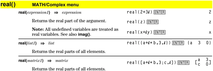
real() MATH/Complex menu
real(expression1) ⇒ expression
Returns the real part of the argument.
Note: All undefined variables are treated as real variables. See also imag().
| Example | Result |
|---|---|
real(2+3i) [ENTER] |
2 |
real(z) [ENTER] |
z |
real(x+i·y) [ENTER] |
x |
real(list1) ⇒ list
Returns the real parts of all elements.
| Example | Result |
|---|---|
real({a+i·b,3,i}) [ENTER] |
{a 3 0} |
real(matrix1) ⇒ matrix
Returns the real parts of all elements.
| Example | Result |
|---|---|
real([a+i·b,3;c,i]) [ENTER] |
[a 3] [c 0] |
▸Rect MATH/Matrix/Vector ops menu
vector ▸Rect
Displays vector in rectangular form [x, y, z]. The vector must be of dimension 2 or 3 and can be a row or a column.
Note: ▸Rect is a display-format instruction, not a conversion function. You can use it only at the end of an entry line, and it does not update ans.
Note: See also ▸Polar.
| Example | Result |
|---|---|
[3,∠π/4,∠π/6] ▸Rect [ENTER] |
[3·√□/□ 3·√□/□ 3·√□/□] |
[a,∠b,∠c] [ENTER] |
[a·cos(b)·sin(c) a·sin(b)·sin(c) a·cos(c)] |
complexValue ▸Rect
Displays complexValue in rectangular form a+bi. The complexValue can have any complex form. However, an re^iθ entry causes an error in Degree angle mode.
Note: You must use parentheses for an (r∠θ) polar entry.
| Example | Result |
|---|---|
| In Radian angle mode: | |
4e^(π/3) ▸Rect [ENTER] |
4·e^(π/3) |
(4∠π/3) ▸Rect [ENTER] |
2+2·√3·i |
| In Degree angle mode: | |
(4∠60) ▸Rect [ENTER] |
2+2·√3·i |
Note: To type ▸Rect from the keyboard, press [2nd] [▶] for the ▶ operator. To type ∠, press [2nd] [∠].
Appendix A: Functions and Instructions 489
ref() MATH/Matrix menu
ref(matrix1[, tol]) \Rightarrow matrix
Returns the row echelon form of matrix1.
Optionally, any matrix element is treated as zero if its absolute value is less than tol. This tolerance is used only if the matrix has floating-point entries and does not contain any symbolic variables that have not been assigned a value. Otherwise, tol is ignored.
- If you use \blacktriangleright [ENTER] or set the mode to Exact/Approx=APPROXIMATE, computations are done using floating-point arithmetic.
- If tol is omitted or not used, the default tolerance is calculated as: 5\epsilon^-14 \cdot \max(dim(matrix1)) \cdot rowNorm(matrix1)
Note: See also rref().
\begin{tabular}{ll} ref([-2,-2,0,-6;1,-1,9,-9;-5, & \ 2,4,-4)] [ENTER] & \beginbmatrix -1 & -2/5 & -4/5 & 4/5 \ 0 & 1 & 4/7 & 11/7 \ 0 & 0 & 1 & -62/71 \endbmatrix \ {[}a,b,c;e,f,g\mapstom1 [ENTER] & \beginbmatrix a & b & c \ e & f & g \endbmatrix \ ref(m1) [ENTER] & \beginbmatrix 1 & f/e & g/e \ 0 & 1 & (ag-ce)/(af-be) \endbmatrix \ remain(7,0) [ENTER] & 7 \ remain(7,3) [ENTER] & 1 \ remain(-7,3) [ENTER] & -1 \ remain(7,-3) [ENTER] & 1 \ remain(-7,-3) [ENTER] & -1 \ remain({12,-14,16},{9,7,-5}) & \ \quad [ENTER] & {3 \quad 0 \quad 1} \ remain([9,-7;6,4],[4,3;4,-3]) & \ \quad [ENTER] & \beginbmatrix 1 & -1 \ 2 & 1 \endbmatrix \ \end{tabular}
remain() MATH/Number menu
remain(expression1, expression2) \Rightarrow expression remain(tis1, list2) \Rightarrow list remain(matrix1, matrix2) \Rightarrow matrix
Returns the remainder of the first argument with respect to the second argument as defined by the identities: remain(x,0) = x remain(x,y) = x-y*iPart(x/y)
As a consequence, note that remain(-x,y) = - remain(x,y). The result is either zero or it has the same sign as the first argument.
Note: See also mod().
Rename CATALOG
Rename oldVarName, newVarName
Renames the variable oldVarName as newVarName.
\begin{tabular}{ll} {1,2,3,4}\mapstoL1 [ENTER] & {1,2,3,4} \ Rename L1, list1 [ENTER] & Done \ list1 [ENTER] & {1,2,3,4} \ \end{tabular}
Request CATALOG
Request promptString, var
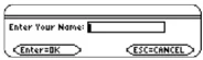
If Request is inside a Dialog...EndDlog construct, it creates an input box for the user to type in data. If it is a stand-alone instruction, it creates a dialog box for this input. In either case, if var contains a string, it is displayed and highlighted in the input box as a default choice. promptString must be \leq 20 characters.
This instruction can be stand-alone or part of a dialog construct.
490 Appendix A: Functions and Instructions
Return CATALOG
Return [expression] Returns expression as the result of the function. Use within a Func...EndFunc block, or Prgm...EndPrgm block.
Note: Use Return without an argument to exit a program.
Note: Enter the text as one long line on the Home screen (without line breaks).
Define factorial(nn)=Func :local answer,count:1⇒answer :For count,1,nn :answer*count⇒answer:EndFor :Return answer:EndFunc ENTER Done factorial(3) ENTER 6
right() MATH/List menu
right(list1[, num]) ⇒ list Returns the rightmost num elements contained in list1.
If you omit num, returns all of list1.
right("Hello",2) ENTER "lo" Returns the rightmost num characters contained in character string sourceString.
If you omit num, returns all of sourceString.
right(x<3) ENTER 3 Returns the right side of an equation or inequality.
rotate() MATH/Base menu
rotate(integer1[, #ofRotations]) ⇒ integer Rotates the bits in a binary integer. You can enter integer1 in any number base; it is converted automatically to a signed, 32-bit binary form. If the magnitude of integer1 is too large for this form, a symmetric modulo operation brings it within the range.
If #of Rotations is positive, the rotation is to the left. If #of Rotations is negative, the rotation is to the right. The default is -1 (rotate right one bit).
For example, in a right rotation:
Each bit rotates right. 0b00000000000001111010110000110101 Rightmost bit rotates to leftmost.
produces: 0b1000000000000111101011000011010
The result is displayed according to the Base mode.
In Bin base mode: rotate(0b1111010110000110101) ENTER 0b1000000000000111101011000011010 rotate(256,1) ENTER 0b1000000000
In Hex base mode: rotate(0h78E) ENTER 0h3C7 rotate(0h78E,-2) ENTER 0h800001E3 rotate(0h78E,2) ENTER 0h1E38
Important: To enter a binary or hexadecimal number, always use the 0b or 0h prefix (zero, not the letter O).
Appendix A: Functions and Instructions 491
rotate(list1[,#ofRotations]) ⇒ list
Returns a copy of list1 rotated right or left by #of Rotations elements. Does not alter list1.
If #of Rotations is positive, the rotation is to the left. If #of Rotations is negative, the rotation is to the right. The default is -1 (rotate right one element).
In Dec base mode:
rotate({1,2,3,4}) ENTER {4 1 2 3}
rotate({1,2,3,4},-2) ENTER {3 4 1 2}
rotate({1,2,3,4},1) ENTER {2 3 4 1}
rotate(string1[,#ofRotations]) ⇒ string
Returns a copy of string1 rotated right or left by #of Rotations characters. Does not alter string1.
If #of Rotations is positive, the rotation is to the left. If #of Rotations is negative, the rotation is to the right. The default is -1 (rotate right one character).
rotate("abcd") ENTER "dabc"
rotate("abcd",-2) ENTER "cdab"
rotate("abcd",1) ENTER "bcda"
round() MATH/Number menu
round(expression1[, digits]) ⇒ expression
Returns the argument rounded to the specified number of digits after the decimal point.
digits must be an integer in the range 0–12. If digits is not included, returns the argument rounded to 12 significant digits.
Note: Display digits mode may affect how this is displayed.
round(1.234567,3) ENTER 1.235
round(list1[, digits]) ⇒ list
Returns a list of the elements rounded to the specified number of digits.
round({π,√(2),ln(2)},4) ENTER {3.1416 1.4142 .6931}
round(matrix1[, digits]) ⇒ matrix
Returns a matrix of the elements rounded to the specified number of digits.
round([ln(5),ln(3);π,e^(1)],1) ENTER
[1.6 1.1] [3.1 2.7]
rowAdd() MATH/Matrix/Row ops menu
rowAdd(matrix1, rIndex1, rIndex2) ⇒ matrix
Returns a copy of matrix1 with row rIndex2 replaced by the sum of rows rIndex1 and rIndex2.
rowAdd([3,4;-3,-2],1,2) ENTER
[3 4] [0 2]
rowAdd([a,b;c,d],1,2) ENTER
[a b ] [a+c b+d]
rowDim() MATH/Matrix/Dimensions menu
rowDim(matrix) ⇒ expression
Returns the number of rows in matrix.
Note: See also colDim().
[1,2;3,4;5,6]→M1 ENTER
rowdim(M1) ENTER
[1 2] [3 4] [5 6] 3
492 Appendix A: Functions and Instructions
rowNorm() MATH/Matrix/Norms menu
rowNorm(matrix) \Rightarrow expression
Returns the maximum of the sums of the absolute values of the elements in the rows in matrix.
Note: All matrix elements must simplify to numbers. See also colNorm().
rowNorm([-5,6,-7;3,4,9;9,-9,-7]) \boxedENTER 25
rowSwap() MATH/Matrix/Row ops menu
rowSwap(matrix1, rIndex1, rIndex2) \Rightarrow matrix
Returns matrix1 with rows rIndex1 and rIndex2 exchanged.
[1,2;3,4;5,6] \rightarrow Mat \boxedENTER
$$ \begin{bmatrix} 1 & 2 \ 3 & 4 \ 5 & 6 \end{bmatrix} $$
rowSwap(Mat,1,3) \boxedENTER
$$ \begin{bmatrix} 5 & 6 \ 3 & 4 \ 1 & 2 \end{bmatrix} $$
RplcPic CATALOG
RplcPic picVar, [row], [column]
Clears the Graph screen and places picture picVar at pixel coordinates (row, column). If you do not want to clear the screen, use RclPic.
picVar must be a picture data type variable. row and column, if included, specify the pixel coordinates of the upper left corner of the picture. Default coordinates are (0, 0).
Note: For less than full-screen pictures, only the area affected by the new picture is cleared.
rref() MATH/Matrix menu
rref(matrix1, [tol]) \Rightarrow matrix
Returns the reduced row echelon form of matrix1.
rref([-2,-2,0,-6;1,-1,9,-9;-5,2,4,-4]) \boxedENTER
$$ \begin{bmatrix} 1 & 0 & 0 & 66/71 \ 0 & 1 & 0 & 147/71 \ 0 & 0 & 1 & -62/71 \end{bmatrix} $$
Optionally, any matrix element is treated as zero if its absolute value is less than tol. This tolerance is used only if the matrix has floating-point entries and does not contain any symbolic variables that have not been assigned a value. Otherwise, tol is ignored.
- If you use \boxedALPHA \boxedENTER or set the mode to Exact/Approx=APPROXIMATE, computations are done using floating-point arithmetic.
- If tol is omitted or not used, the default tolerance is calculated as: 5\epsilon^-14 * \max(\dim(matrix1)) * rowNorm(matrix1)
Note: See also ref().
rref([a,b,x;c,d,y]) \boxedENTER
$$ \begin{bmatrix} 1 & 0 & \frac{d \cdot x - b \cdot y}{a \cdot d - b \cdot c} \ 0 & 1 & \frac{-(c \cdot x - a \cdot y)}{a \cdot d - b \cdot c} \end{bmatrix} $$
Appendix A: Functions and Instructions 493
Send CATALOG
Send list
CBL 2™/CBL™ (Calculator-Based Laboratory™) or CBR™ (Calculator-Based Ranger™) instruction. Sends list to the link port.
Program segment: : :Send {1,0} :Send {1,2,1} :
SendCalc CATALOG
SendCalc var
Sends variable var to the link port, where another unit linked to that port can receive the variable value. The receiving unit must be on the Home screen or must execute GetCalc from a program.
If you send from a TI-89 or TI-92 Plus to a TI-92, an error occurs if the TI-92 executes GetCalc from a program. In this case, the sending unit must use SendChat instead.
Program segment: : :a+b→x :SendCalc x :
SendChat CATALOG
SendChat var
A general alternative to SendCalc, this is useful if the receiving unit is a TI-92 (or for a generic "chat" program that allows either a TI-92 or TI-92 Plus to be used). Refer to SendCalc for more information.
SendChat sends a variable only if that variable is compatible with the TI-92, which is typically true in "chat" programs. However, SendChat will not send an archived variable, a TI-89 graph data base, etc.
Program segment: : :a+b→x :SendChat x :
seq() MATH/List menu
seq(expression, var, low, high[, step]) \Rightarrow list
Increments var from low through high by an increment of step, evaluates expression, and returns the results as a list. The original contents of var are still there after seq() is completed.
var cannot be a system variable.
The default value for step = 1.

494 Appendix A: Functions and Instructions
setFold() CATALOG
setFold(newfolderName) \Rightarrow oldfolderString
Returns the name of the current folder as a string and sets newfolderName as the current folder.
The folder newfolderName must exist.
newFold chris [ENTER] Done setFold(main) [ENTER] "chris" setFold(chris)\Rightarrowoldfoldr [ENTER] "main" 1\Rightarrowa [ENTER] 1 setFold(#oldfoldr) [ENTER] "chris" a [ENTER] a chris\a [ENTER] 1
setGraph() CATALOG
setGraph(modeNameString, settingString) \Rightarrow string
Sets the Graph mode modeNameString to settingString, and returns the previous setting of the mode. Storing the previous setting lets you restore it later.
modeNameString is a character string that specifies which mode you want to set. It must be one of the mode names from the table below.
settingString is a character string that specifies the new setting for the mode. It must be one of the settings listed below for the specific mode you are setting.
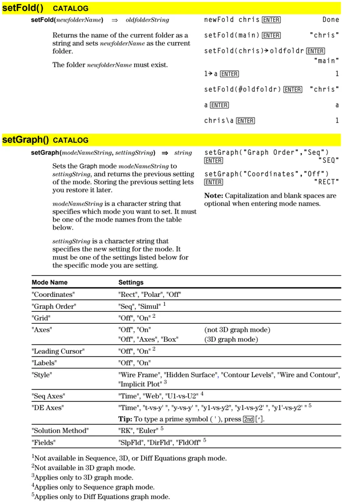
setGraph("Graph Order","Seq") [ENTER] "SEQ" setGraph("Coordinates","Off") [ENTER] "RECT"
Note: Capitalization and blank spaces are optional when entering mode names.
\begin{tabular}{ll} Mode Name & Settings \ \hline "Coordinates" & "Rect", "Polar", "Off" \ "Graph Order" & "Seq", "Simul" $^{1}$ \ "Grid" & "Off", "On" $^{2}$ \ "Axes" & "Off", "On" \quad (not 3D graph mode) \ & "Off", "Axes", "Box" \quad (3D graph mode) \ "Leading Cursor" & "Off", "On" $^{2}$ \ "Labels" & "Off", "On" \ "Style" & "Wire Frame", "Hidden Surface", "Contour Levels", "Wire and Contour", \ & "Implicit Plot" $^{3}$ \ "Seq Axes" & "Time", "Web", "U1-vs-U2" $^{4}$ \ "DE Axes" & "Time", "t-vs-y' ", "y-vs-y' ", "y1-vs-y2", "y1-vs-y2' ", "y1'-vs-y2' " $^{5}$ \ & \textbf{Tip:} To type a prime symbol ( '), press [2nd][']. \ "Solution Method" & "RK", "Euler" $^{5}$ \ "Fields" & "SlpFld", "DirFld", "FldOff" $^{5}$ \ \end{tabular}
$^{1}$Not available in Sequence, 3D, or Diff Equations graph mode. $^{2}$Not available in 3D graph mode. $^{3}$Applies only to 3D graph mode. $^{4}$Applies only to Sequence graph mode. $^{5}$Applies only to Diff Equations graph mode.
Appendix A: Functions and Instructions 495
setMode() CATALOG
\begin{tabular}{p{0.5\textwidth} p{0.45\textwidth}} setMode(modeNameString, settingString) \Rightarrow string \newline setMode(list) \Rightarrow stringList & setMode("Angle","Degree") \newline \textbf{ENTER} \quad "RADIAN" \ Sets mode modeNameString to the new setting settingString, and returns the current setting of that mode. & sin(45) \textbf{ENTER} \quad \frac\sqrt22 \ modeNameString is a character string that specifies which mode you want to set. It must be one of the mode names from the table below. & setMode("Angle","Radian") \newline \textbf{ENTER} \quad "DEGREE" \ settingString is a character string that specifies the new setting for the mode. It must be one of the settings listed below for the specific mode you are setting. & sin(\pi/4) \textbf{ENTER} \quad \frac\sqrt22 \ list contains pairs of keyword strings and will set them all at once. This is recommended for multiple-mode changes. The example shown may not work if each of the pairs is entered with a separate setMode() in the order shown. & setMode("Display Digits", "Fix 2") \textbf{ENTER} \quad "FLOAT" \ Use setMode(var) to restore settings saved with getMode("ALL")\rightarrowvar. & \pi \blacktriangleright \textbf{ENTER} \quad 3.14 \ \textbf{Note:} To set or return information about the Unit System mode, use setUnits() or getUnits() instead of setMode() or getMode(). & setMode ("Display Digits", "Float") \textbf{ENTER} \quad "FIX 2" \ & \pi \blacktriangleright \textbf{ENTER} \quad 3.141... \ & setMode({"Split Screen", "Left-Right","Split 1 App", "Graph","Split 2 App","Table"}) \newline \textbf{ENTER} \ & \quad {"Split 2 App" "Graph" \quad "Split 1 App" "Home" \quad "Split Screen" "FULL"} \ & \textbf{Note:} Capitalization and blank spaces are optional when entering mode names. Also, the results in these examples may be different on your unit. \
- \multicolumn{2}{l}{\textbf{Mode Name} \quad \quad \quad \quad \quad \quad \quad \quad \quad \quad \quad \quad \quad \quad \quad \quad \quad \quad \quad \quad \quad \quad \quad \quad \quad \quad \quad \quad \quad \quad \quad \quad \quad \quad \quad \quad \quad \quad \quad \quad \quad \quad \quad \quad \quad \quad \quad \quad \quad \quad \quad ........ \textbf{Settings}} \ \multicolumn{2}{l}{----------------------------------------------} \ \multicolumn{2}{l}{"Graph" \quad \quad \quad \quad \quad \quad \quad \quad \quad \quad \quad \quad \quad \quad \quad \quad \quad \quad \quad \quad \quad \quad \quad \quad \quad \quad \quad "Function", "Parametric", "Polar", "Sequence", "3D", "Diff Equations"} \ \multicolumn{2}{l}{"Display Digits" \quad \quad \quad \quad \quad \quad \quad \quad \quad \quad \quad \quad \quad \quad \quad \quad \quad \quad \quad \quad \quad \quad \quad \quad "Fix 0", "Fix 1", ..., "Fix 12", "Float", "Float 1", ..., "Float 12"} \
- \multicolumn{2}{l}{"Angle" \quad \quad \quad \quad \quad \quad \quad \quad \quad \quad \quad \quad \quad \quad \quad \quad \quad \quad \quad \quad \quad \quad \quad \quad \quad \quad \quad \quad \quad \quad \quad \quad \quad \quad \quad \quad \quad \quad \quad \quad \quad \quad \quad \quad \quad \quad \quad \quad \quad \quad \quad \quad \quad \quad \quad \quad \quad \quad \quad \quad \quad \quad \quad \quad \ ........ "Radian", "Degree"} \
- \multicolumn{2}{l}{"Exponential Format" \quad \quad \quad \quad \quad \quad \quad \quad \quad \quad \quad \quad \quad \quad \quad \quad \quad \quad \quad \quad \quad \quad \quad \quad \quad \quad \quad \quad \quad \quad \quad \quad \quad \quad \quad \quad \quad \quad \quad \quad \quad \quad \quad \quad \quad \quad \quad \quad \quad \quad \quad \quad \quad \quad \quad \quad \quad \quad \quad \quad \quad \quad \quad \quad \quad \quad \quad \quad \quad \quad \quad \ ........
setTable() CATALOG
setTable(modeNameString, settingString) \Rightarrow string
Sets the table parameter modeNameString to settingString, and returns the previous setting of the parameter. Storing the previous setting lets you restore it later.
modeNameString is a character string that specifies which parameter you want to set. It must be one of the parameters from the table below.
settingString is a character string that specifies the new setting for the parameter. It must be one of the settings listed below for the specific parameter you are setting.
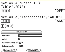
Note: Capitalization and blank spaces are optional when entering parameters.
\begin{tabular}{ll} Parameter Name & Settings \ "Graph $<->$ Table" & "Off", "On" \ "Independent" & "Auto", "Ask" \ \end{tabular}
setUnits() CATALOG
setUnits(list1) \Rightarrow list
Sets the default units to the values specified in list1, and returns a list of the previous defaults.
- To specify the built-in SI (metric) or ENG/US system, list1 uses the form: {"SI"} or {"ENG/US"}
- To specify a custom set of default units, list1 uses the form: {"CUSTOM", "cat1", "unit1"[, "cat2", "unit2", ...]} where each cat and unit pair specifies a category and its default unit. (You can specify built-in units only, not user-defined units.) Any category not specified will use its previous custom unit.
- To return to the previous custom default units, list1 uses the form: {"CUSTOM"}
If you want different defaults depending on the situation, create separate lists and save them to unique list names. To use a set of defaults, specify that list name in setUnits().
You can use setUnits() to restore settings previously saved with setUnits() \rightarrow var or with getUnits() \rightarrow var.
All unit names must begin with an underscore _.
TI-89: [ ] TI-92 Plus: [2nd] [ ]
You can also select units from a menu by pressing:
TI-89: [2nd] [UNITS] TI-92 Plus: [ ] [UNITS]
setUnits({"SI"}) [ENTER] {"SI" "Area" "NONE" "Capacitance" "_F" ...}
setUnits({"CUSTOM","Length", "_cm","Mass","_gm"}) [ENTER] {"SI" "Length" "_m" "Mass" "_kg" ...}
Note: Your screen may display different units.
Appendix A: Functions and Instructions 497
Shade CATALOG
Shade expr1, expr2, [xlow], [xhigh], [pattern], [patRes]
Displays the Graph screen, graphs expr1 and expr2, and shades areas in which expr1 is less than expr2. (expr1 and expr2 must be expressions that use x as the independent variable.)
xlow and xhigh, if included, specify left and right boundaries for the shading. Valid inputs are between xmin and xmax. Defaults are xmin and xmax.
pattern specifies one of four shading patterns: 1 = vertical (default) 2 = horizontal 3 = negative-slope 45° 4 = positive-slope 45°
patRes specifies the resolution of the shading patterns: 1= solid shading 2= 1 pixel spacing (default) 3= 2 pixels spacing ... 10= 9 pixels spacing
Note: Interactive shading is available on the Graph screen through the Shade instruction. Automatic shading of a specific function is available through the Style instruction. Shade is not valid in 3D graphing mode.
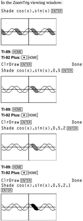
In the ZoomTrig viewing window:
Shade cos(x),sin(x) ENTER
TI-89: HOME TI-92 Plus: [HOME]
ClrDraw ENTER Done Shade cos(x),sin(x),0,5 ENTER
TI-89: HOME TI-92 Plus: [HOME]
ClrDraw ENTER Done Shade cos(x),sin(x),0,5,2 ENTER
TI-89: HOME TI-92 Plus: [HOME]
ClrDraw ENTER Done Shade cos(x),sin(x),0,5,2,1 ENTER
498 Appendix A: Functions and Instructions
shift()
CATALOG
shift(integer1[,#ofShifts]) → integer
Shifts the bits in a binary integer. You can enter integer1 in any number base; it is converted automatically to a signed, 32-bit binary form. If the magnitude of integer1 is too large for this form, a symmetric modulo operation brings it within the range.
If #ofShifts is positive, the shift is to the left. If #ofShifts is negative, the shift is to the right. The default is -1 (shift right one bit).
In a right shift, the rightmost bit is dropped and 0 or 1 is inserted to match the leftmost bit. In a left shift, the leftmost bit is dropped and 0 is inserted as the rightmost bit.
For example, in a right shift:
→ Each bit shifts right. 0b000000000000001111010110000110101 ↑ Inserts 0 if leftmost bit is 0, or 1 if leftmost bit is 1. Dropped produces: 0b00000000000000111101011000011010
The result is displayed according to the Base mode. Leading zeros are not shown.
In Bin base mode:
shift(0b1111010110000110101) ENTER 0b111101011000011010 shift(256,1) ENTER 0b1000000000
In Hex base mode:
shift(0h78E) ENTER 0h3C7 shift(0h78E,-2) ENTER 0h1E3 shift(0h78E,2) ENTER 0h1E38
Important: To enter a binary or hexadecimal number, always use the 0b or 0h prefix (zero, not the letter O).
shift(list1[,#ofShifts]) → list
Returns a copy of list1 shifted right or left by #ofShifts elements. Does not alter list1.
If #ofShifts is positive, the shift is to the left. If #ofShifts is negative, the shift is to the right. The default is -1 (shift right one element).
Elements introduced at the beginning or end of list by the shift are set to the symbol “undef”.
In Dec base mode:
shift({1,2,3,4}) ENTER {undef 1 2 3} shift({1,2,3,4},-2) ENTER {undef undef 1 2} shift({1,2,3,4},1) ENTER {2 3 4 undef}
shift(string1[,#ofShifts]) → string
Returns a copy of string1 shifted right or left by #ofShifts characters. Does not alter string1.
If #ofShifts is positive, the shift is to the left. If #ofShifts is negative, the shift is to the right. The default is -1 (shift right one character).
Characters introduced at the beginning or end of string by the shift are set to a space.
shift("abcd") ENTER " abc" shift("abcd",-2) ENTER " ab" shift("abcd",1) ENTER "bcd "
Appendix A: Functions and Instructions 499
ShowStat CATALOG
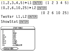
ShowStat Displays a dialog box containing the last computed statistics results if they are still valid. Statistics results are cleared automatically if the data to compute them has changed.
Use this instruction after a statistics calculation, such as LinReg.
(1,2,3,4,5) \rightarrow L1 [ENTER] {1 2 3 4 5} (0,2,6,10,25) \rightarrow L2 [ENTER] {0 2 6 10 25} TwoVar L1,L2 [ENTER] ShowStat [ENTER]
sign() MATH/Number menu
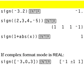
sign(expression1) \Rightarrow expression sign(list1) \Rightarrow list sign(matrix1) \Rightarrow matrix
For real and complex expression1, returns expression1/abs(expression1) when expression1 \neq 0.
Returns 1 if expression1 is positive. Returns -1 if expression1 is negative. sign(0) returns ±1 if the complex format mode is REAL; otherwise, it returns itself. sign(0) represents the unit circle in the complex domain.
For a list or matrix, returns the signs of all the elements.
sign(-3.2) [ENTER] -1. sign({2,3,4,-5}) [ENTER] {1 1 1 -1} sign(1+abs(x)) [ENTER] 1
If complex format mode is REAL: sign([-3,0,3]) [ENTER] [-1 ±1 1]
simult() MATH/Matrix menu
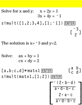
simult(coeffMatrix, constVector[, tol]) \Rightarrow matrix
Returns a column vector that contains the solutions to a system of linear equations.
coeffMatrix must be a square matrix that contains the coefficients of the equations.
constVector must have the same number of rows (same dimension) as coeffMatrix and contain the constants.
Optionally, any matrix element is treated as zero if its absolute value is less than tol. This tolerance is used only if the matrix has floating-point entries and does not contain any symbolic variables that have not been assigned a value. Otherwise, tol is ignored.
- If you use [\blacklozenge][ENTER] or set the mode to Exact/Approx=APPROXIMATE, computations are done using floating-point arithmetic.
- If tol is omitted or not used, the default tolerance is calculated as: 5E-14 * max(dim(coeffMatrix)) * rowNorm(coeffMatrix)
Solve for x and y: x + 2y = 1 3x + 4y = -1
simult([1,2;3,4],[1;-1]) [ENTER] [[-3] [ 2]]
The solution is x=-3 and y=2.
Solve: ax + by = 1 cx + dy = 2
[a,b;c,d] \rightarrow matx1 [ENTER] [[a b] [c d]] simult(matx1,[1;2]) [ENTER] [[-(2·b-d)] / [a·d-b·c]] [[2·a-c] / [a·d-b·c]]
500 Appendix A: Functions and Instructions
simult(coeffMatrix, constMatrix[, tol]) ⇒ matrix
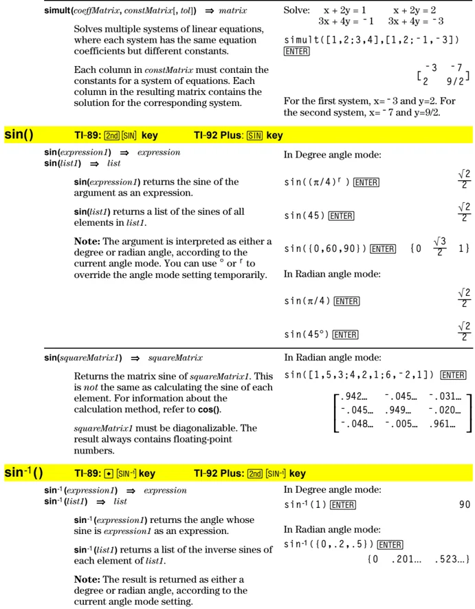
Solves multiple systems of linear equations, where each system has the same equation coefficients but different constants.
Each column in constMatrix must contain the constants for a system of equations. Each column in the resulting matrix contains the solution for the corresponding system.
Solve: x + 2y = 1 x + 2y = 2 3x + 4y = -1 3x + 4y = -3
simult([1,2;3,4],[1,2;-1,-3]) ENTER
[ -3 -7 ] [ 2 9/2 ]
For the first system, x= -3 and y=2. For the second system, x= -7 and y=9/2.
sin()
TI-89: [2nd] [SIN] key TI-92 Plus: [SIN] key
sin(expression1) ⇒ expression
sin(list1) ⇒ list
sin(expression1) returns the sine of the argument as an expression.
sin(list1) returns a list of the sines of all elements in list1.
Note: The argument is interpreted as either a degree or radian angle, according to the current angle mode. You can use ° or ᵣ to override the angle mode setting temporarily.
In Degree angle mode:
sin((π/4)ᵣ) ENTER √□/□
sin(45) ENTER √□/□
sin({0,60,90}) ENTER {0 √□/□ 1}
In Radian angle mode:
sin(π/4) ENTER √□/□
sin(45°) ENTER √□/□
sin(squareMatrix1) ⇒ squareMatrix
Returns the matrix sine of squareMatrix1. This is not the same as calculating the sine of each element. For information about the calculation method, refer to cos().
squareMatrix1 must be diagonalizable. The result always contains floating-point numbers.
In Radian angle mode:
sin([1,5,3;4,2,1;6,-2,1]) ENTER
[ .942... -.045... -.031... ]
[ -.045... .949... -.020... ]
[ -.048... -.005... .961... ]
sin⁻¹()
TI-89: [♦] [SIN⁻¹] key TI-92 Plus: [2nd] [SIN⁻¹] key
sin⁻¹(expression1) ⇒ expression
sin⁻¹(list1) ⇒ list
sin⁻¹(expression1) returns the angle whose sine is expression1 as an expression.
sin⁻¹(list1) returns a list of the inverse sines of each element of list1.
Note: The result is returned as either a degree or radian angle, according to the current angle mode setting.
In Degree angle mode:
sin⁻¹(1) ENTER 90
In Radian angle mode:
sin⁻¹({0,.2,.5}) ENTER
{0 .201... .523...}
Appendix A: Functions and Instructions 501
sin⁻¹(squareMatrix1) ⇒ squareMatrix
Returns the matrix inverse sine of squareMatrix1. This is not the same as calculating the inverse sine of each element. For information about the calculation method, refer to cos().
squareMatrix1 must be diagonalizable. The result always contains floating-point numbers.
In Radian angle mode and Rectangular complex format mode:
sin⁻¹([1,5,3;4,2,1;6,-2,1]) ENTER
[ -.164...-.064...·i 1.490...-2.105...·i ... ] [ .725...-1.515...·i .947...-.778...·i ... ] [ 2.083...-2.632...·i -1.790...+1.271...·i ... ]
sinh() MATH/Hyperbolic menu
sinh(expression1) ⇒ expression
sinh(list1) ⇒ list
sinh (expression1) returns the hyperbolic sine of the argument as an expression.
sinh (list) returns a list of the hyperbolic sines of each element of list1.
sinh(1.2) ENTER 1.509...
sinh({0,1.2,3.}) ENTER {0 1.509... 10.017...}
sinh(squareMatrix1) ⇒ squareMatrix
Returns the matrix hyperbolic sine of squareMatrix1. This is not the same as calculating the hyperbolic sine of each element. For information about the calculation method, refer to cos().
squareMatrix1 must be diagonalizable. The result always contains floating-point numbers.
In Radian angle mode:
sinh([1,5,3;4,2,1;6,-2,1])
ENTER
[ 360.954 305.708 239.604 ] [ 352.912 233.495 193.564 ] [ 298.632 154.599 140.251 ]
sinh⁻¹() MATH/Hyperbolic menu
sinh⁻¹(expression1) ⇒ expression
sinh⁻¹(list1) ⇒ list
sinh⁻¹(expression1) returns the inverse hyperbolic sine of the argument as an expression.
sinh⁻¹(list1) returns a list of the inverse hyperbolic sines of each element of list1.
sinh⁻¹(0) ENTER 0
sinh⁻¹({0,2.1,3}) ENTER {0 1.487... sinh⁻¹(3)}
sinh⁻¹(squareMatrix1) ⇒ squareMatrix
Returns the matrix inverse hyperbolic sine of squareMatrix1. This is not the same as calculating the inverse hyperbolic sine of each element. For information about the calculation method, refer to cos().
squareMatrix1 must be diagonalizable. The result always contains floating-point numbers.
In Radian angle mode:
sinh⁻¹([1,5,3;4,2,1;6,-2,1])
ENTER
[ .041... 2.155... 1.158... ] [ 1.463... .926... .112... ] [ 2.750... -1.528... .572... ]
502 Appendix A: Functions and Instructions