Combining Multiple Units
You may need to combine two or more units from different categories.
For example, suppose you want to enter a velocity in meters per second. In the UNITS dialog box, however, the Velocity category does not contain this unit.

Tip: Create a user-defined unit (page 88) for frequently used combinations.
You can enter meters per second by combining _m and _s from the Length and Time categories, respectively.
3*9.8_m/_s Combine the units _m and _s. There is no pre-defined _m/_s unit.
Using Parentheses with Units in a Calculation
In a calculation, you may need to use parentheses ( ) to group a value and its units so that they are evaluated properly. This is particularly true for division problems. For example:
Tip: If you have any doubt about how a value and its units will be evaluated, group them within parentheses ( ).
To calculate: Enter:
100_m / 2_s 100_m/(2_s) 50._m/_s You must use parentheses for (2_s). This is important for division.
If you omit the parentheses, you will get unexpected units. For example:
100_m/2_s 50._m*_s
Here’s why you get unexpected units if you do not use parentheses. In a calculation, a unit is treated similar to a variable. For example:
100_m is treated as 100*_m and 2_s is treated as 2*_s
Without parentheses, the entry is calculated as:
$100*_m / 2*_s = 100*_m/2 *_s = 50.\cdot_m\cdot_s$
84 Chapter 4: Constants and Measurement Units

Converting from One Unit to Another
You can convert from one unit to another in the same category, including any user-defined units (page 88).
For All Units Except Temperature
If you use a unit in a calculation, it is converted and displayed automatically in the current default unit for that category, unless you use the ▶ conversion operator as described later. The following examples assume that your default units are set to the SI system of metric units (page 87).
Note: For a list of pre- defined units, see page 89.
Tip: From the UNITS dialog box, you can select available units from a menu.
To multiply 20 times 6 kilometers.
20*6_km
Shown in the default unit for Length, (_m in SI system).
If you want to convert to a unit other than the default, use the ▶ conversion operator.
expression_unit1 ▶ _unit2
For ▶, press [2nd] [▶].
To convert 4 light years to kilometers:
4_ltyr \blacktriangleright _km
To convert 186000 miles/second to kilometers/hour:
186000_mi/_s \blacktriangleright _km/_hr
If an expression uses a combination of units, you can specify a conversion for some of the units only. Any units for which you do not specify a conversion will be displayed according to your defaults.
To convert 186000 miles/second from miles to kilometers:
186000_mi/_s \blacktriangleright _km
Because a Time conversion is not specified, it is shown in its default unit (_s in this example).
To convert 186000 miles/second from seconds to hours:
186000_mi/_s \blacktriangleright 1/_hr
Because a Length conversion is not specified, it is shown in its default unit (_m in this example).
Chapter 4: Constants and Measurement Units 85


To enter meters per second squared: 27_m/_s^2

To convert meters per second squared from seconds to hours: 27_m/_s^2►1/_hr^2
For Temperature Values
To convert a temperature value, you must use tmpCnv() instead of the ► operator. tmpCnv(expression_°tempUnit1, _°tempUnit2) For °, press [2nd] [°].
For example, to convert 100_°C to °F: tmpCnv(100°c, _°f)
For Temperature Ranges
For \Delta, press: TI-89: [\blacklozenge] [1] [↑] [D] TI-92 Plus: [2nd] [G] [↑] [D]
To convert a temperature range (the difference between two temperature values), use \Delta.tmpCnv(). \Delta.tmpCnv(expression_°tempUnit1, _°tempUnit2)
For example, to convert a 100_°C range to its equivalent range in _°F: \Delta.tmpCnv(100_°c, _°f)
86 Chapter 4: Constants and Measurement Units


Setting the Default Units for Displayed Results
All results involving units are displayed in the default unit for that category. For example, if the default unit for Length is _m, any length result is displayed in meters (even if you entered _km or _ft in the calculation).
If You're Using the SI or ENG/US System
The SI and ENG/US systems of measurement (set from Page 3 of the MODE screen) use built-in default units, which you cannot change.
To find the default units for these systems, refer to page 89.
If Unit System=SI or ENG/US, the Custom Units item is dimmed. You cannot set a default for individual categories.
Setting Custom Defaults
To set custom defaults:
- Press MODE F3 3 to set Unit System = CUSTOM.
- Press \Theta to highlight SET DEFAULTS.
- Press 1 to display the CUSTOM UNIT DEFAULTS dialog box.
- For each category, you can highlight its default, press 1, and select a unit from the list.
- Press [ENTER] twice to save your changes and exit the MODE screen.
Note: You can also use setUnits() or getUnits() to set or return information about default units. Refer to Appendix A.
Tip: When the CUSTOM UNIT DEFAULTS dialog box first appears, it shows the current default units.
You can also move the cursor by typing the first letter of a unit.
What is the NONE Default?
Many categories let you select NONE as the default unit.
This means that results in that category are displayed in the default units of its components.
For example, Area = Length$^2$, so Length is the component of Area.
Note: NONE is not available for base categories such as Length and Mass that have no components.
- If the defaults are Area = _acre and Length = _m (meters), area results are shown with _acre units.
- If you set Area = NONE, area results are shown with _m$^2$ units.
Chapter 4: Constants and Measurement Units 87


Creating Your Own User-Defined Units
In any category, you can expand the list of available units by defining a new unit in terms of one or more pre-defined units. You can also use “standalone” units.
Why Use Your Own Units?
Some example reasons to create a unit are:
- You want to enter length values in dekameters. Define 10_m as a new unit named _dm.
- Instead of entering _m/_s$^2$ as an acceleration unit, you define that combination of units as a single unit named _ms2.
- You want to calculate how many times someone blinks. You can use _blinks as a valid unit without defining it. This “standalone” unit is treated similar to a variable that is not defined. For instance, 3_blinks is treated the same as 3a.
Note: If you create a user-defined unit for an existing category, you can select it from the UNITS dialog box menu. But you cannot use MODE to select the unit as a default for displayed results.
Rules for User-Defined Unit Names
The naming rules for units are similar to variables.
- Can have up to 8 characters. First character must be an underscore. For , press: TI-89: [◄] [] TI-92 Plus: [2nd] [_]
- Second character can be any valid variable name character except _ or a digit. For example, _9f is not valid.
- Remaining characters (up to 6) can be any valid variable name character except an underscore.
Defining a Unit
Define a unit the same way you store to a variable.
definition \rightarrow _newUnit For \rightarrow, press [STO\blacktriangleright].
Note: User-defined units are displayed in lowercase characters, regardless of the case you use to define them.
Note: User-defined units such as _dm are stored as variables. You can delete them the same as you would any variable.
For example, to define a dekameter unit: 10_m \rightarrow _dm
To define an acceleration unit: _m/_s^2 \rightarrow _ms2

Assuming unit defaults for Length and Time are set to _m and _s.
To calculate 195 blinks in 5 minutes as _blinks/_min: 195_blinks/(5_min)
Assuming unit default for Time is set to _s.
88 Chapter 4: Constants and Measurement Units
List of Pre-Defined Constants and Units
This section lists the pre-defined constants and units by category. You can select any of these from the UNITS dialog box. If you use [MODE] to set default units, note that categories with only one defined unit are not listed.
Defaults for SI and ENG/US
The SI and ENG/US systems of measurement use built-in default units. In this section, the built-in defaults are indicated by (SI) and (ENG/US). In some categories, both systems use the same default.
For a description of the NONE default, refer to page 87. Notice that some categories do not have default units.
Constants
Note: The TI-89 / TI-92 Plus simplifies unit expressions and displays results according to your default units. Therefore, constant values displayed on your screen may appear different from the values in this table.
Tip: For Greek characters, refer to Shortcut Keys (inside front and back covers).
- _c ........ speed of light ........ 2.99792458E8_m/_s
- _Cc ........ coulomb constant ........ 8.9875517873682E9_N•_m²/_coul²
- _g ........ acceleration of gravity ........ 9.80665_m/_s²
- _Gc ........ gravitational constant ........ 6.67259E-11_m³/_kg/_s²
- _h ........ Planck’s constant ........ 6.6260755E-34_J•_s
- k ........ Boltzmann’s constant ........ 1.380658E-23_J/°K
- _Me ........ electron rest mass ........ 9.1093897E-31_kg
- _Mn ........ neutron rest mass ........ 1.6749286E-27_kg
- _Mp ........ proton rest mass ........ 1.6726231E-27_kg
- _Na ........ Avogadro’s number ........ 6.0221367E23/_mol
- _q ........ electron charge ........ 1.60217733E-19_coul
- _Rb ........ Bohr radius ........ 5.29177249E-11_m
- _Rc ........ molar gas constant ........ 8.31451_J/mol/°K
- _Rdb ........ Rydberg constant ........ 10973731.53413/_m
- _Vm ........ molar volume ........ 2.241409E-2_m³/_mol
- _ε0 ........ permittivity of a vacuum ........ 8.8541878176204E-12_F/_m
- _σ ........ Stefan-Boltzmann constant ........ 5.6705119E-8_W/m²/°K⁴
- _φ0 ........ magnetic flux quantum ........ 2.0678346161E-15_Wb
- _μ0 ........ permeability of a vacuum ........ 1.2566370614359E-6_N/_A²
- _μb ........ Bohr magneton ........ 9.2740154E-24_J•_m²/_Wb
Length
-
_Ang ........ angstrom
-
_au ........ astronomical unit
-
_cm ........ centimeter
-
_fath ........ fathom
-
_fm ........ fermi
-
_ft ........ foot (ENG/US)
-
_in ........ inch
-
_km ........ kilometer
-
_ltyr ........ light year
-
_m ........ meter (SI)
-
_mi ........ mile
-
_mil ........ 1/1000 inch
-
_mm ........ millimeter
-
_Nmi ........ nautical mile
-
_pc ........ parsec
-
_rod ........ rod
-
_yd ........ yard
-
_μ ........ micron
-
_Å ........ angstrom
Area
- _acre ........ acre
- _ha ........ hectare
NONE (SI) (ENG/US)
Chapter 4: Constants and Measurement Units 89
Volume
- _cup ........ cup
- _floz ........ fluid ounce _flozUK .. British fluid ounce
- _gal ........ gallon
- _galUK ........ British gallon
- _l ........ liter
- _ml ........ milliliter
- _pt ........ pint
- _qt ........ quart
- _tbsp ........ tablespoon
- _tsp ........ teaspoon NONE (SI) (ENG/US)
Time
- _day ........ day
- _hr ........ hour
- _min ........ minute
- _ms ........ millisecond
- _ns ........ nanosecond
- _s ........ second (SI) (ENG/US)
- _week ........ week
- _yr ........ year
- _μs ........ microsecond
Velocity
- _knot ........ knot
- _kph ........ kilometers per hour
- _mph ........ miles per hour NONE (SI) (ENG/US)
Acceleration no pre-defined units
Temperature
- _°C ........ °Celsius For °, press [2nd] [°].
- _°F ........ °Fahrenheit
- _°K ........ °Kelvin
- _°R ........ °Rankine (no default)
Luminous Intensity
- _cd ........ candela (no default)
Amount of Substance
- _mol ........ mole (no default)
Mass
- _amu ........ atomic mass unit
- _gm ........ gram
- _kg ........ kilogram (SI)
- _lb ........ pound (ENG/US)
- _mg ........ milligram
- _mton ........ metric ton
- _oz ........ ounce
- _slug ........ slug
- _ton ........ ton
- _tonne ........ metric ton _tonUK ... long ton
Force
- _dyne ........ dyne
- _kgf ........ kilogram force
- _lbf ........ pound force (ENG/US)
- _N ........ newton (SI)
- _tonf ........ ton force
Energy
- _Btu ........ British thermal unit (ENG/US)
- _cal ........ calorie
- _erg ........ erg
- _eV ........ electron volt
- _ftlb ........ foot-pound
- _J ........ joule (SI)
- _kcal ........ kilocalorie
- _kWh ........ kilowatt-hour
- _latm ........ liter-atmosphere
Power
- _hp ........ horsepower (ENG/US)
- _kW ........ kilowatt
- _W ........ watt (SI)
90 Chapter 4: Constants and Measurement Units
Pressure
- _atm ........ atmosphere
- _bar ........ bar _inH2O ... inches of water
- _inHg ........ inches of mercury _mmH2O.. millimeters of water _mmHg... millimeters of mecury
- _Pa ........ pascal (SI)
- _psi ........ pounds per square inch (ENG/US)
- _torr ........ millimeters of mecury
Viscosity, Kinematic
- _St ........ stokes
Viscosity, Dynamic
- _P ........ poise
Frequency
- _GHz ........ gigahertz
- _Hz ........ hertz (SI) (ENG/US)
- _kHz ........ kilohertz
- _MHz ........ megahertz
Electric Current
- _A ........ ampere (SI) (ENG/US)
- _kA ........ kiloampere
- _mA ........ milliampere
- _µA ........ microampere
Charge
- _coul ........ coulomb (SI) (ENG/US)
Potential
- _kV ........ kilovolt
- _mV ........ millivolt
- _V ........ volt (SI) (ENG/US)
- _volt ........ volt
Resistance
- _kΩ ........ kilo ohm
- _MΩ ........ megaohm
- _ohm ........ ohm
- _Ω ........ ohm (SI) (ENG/US)
Conductance
- _mho ........ mho (ENG/US) _mmho ... millimho _siemens..siemens (SI)
- _µmho ........ micromho
Capacitance
- _F ........ farad (SI) (ENG/US)
- _nF ........ nanofarad
- _pF ........ picofarad
- _µF ........ microfarad
Mag Field Strength
- _Oe ........ oersted NONE (SI) (ENG/US)
Mag Flux Density
- _Gs ........ gauss
- _T ........ tesla (SI) (ENG/US)
Magnetic Flux
- _Wb ........ weber (SI) (ENG/US)
Inductance
- _henry ........ henry (SI) (ENG/US)
- _mH ........ millihenry
- _nH ........ nanohenry
- _µH ........ microhenry
Chapter 4: Constants and Measurement Units 91
92 Chapter 4: Constants and Measurement Units
Additional Home Screen Topics
5
- Saving the Home Screen Entries as a Text Editor Script ........ 94
- Cutting, Copying, and Pasting Information ........ 95
- Creating and Evaluating User-Defined Functions ........ 97
- Using Folders to Store Independent Sets of Variables ........ 100
- If an Entry or Answer Is “Too Big” ........ 103
To help you get started using the TI-89 / TI-92 Plus as quickly as possible, Chapter 2 described the basic operations of the Home screen.
This chapter describes additional operations that can help you use the Home screen more effectively.

Because this chapter consists of various stand-alone topics, it does not start with a “preview” example.
Chapter 5: Additional Home Screen Topics 93

Saving the Home Screen Entries as a Text Editor Script
To save all the entries in the history area, you can save the Home screen to a text variable. When you want to reexecute those entries, use the Text Editor to open the variable as a command script.
Saving the Entries in the History Area
From the Home screen:
- Press
F1and select 2:Save Copy As.

- Specify a folder and text variable that you want to use to store the entries.

| Item | Description |
|---|---|
| Type | Automatically set as Text and cannot be changed. |
| Folder | Shows the folder in which the text variable will be stored. To use a different folder, press ◊ to display a menu of existing folders. Then select a folder. |
| Variable | Type a valid, unused variable name. |
- Press
ENTER(after typing in an input box such as Variable, pressENTERtwice).
Note: Only the entries are saved, not the answers.
Note: For information about folders, refer to page 100.
Restoring the Saved Entries
Because the entries are stored in a script format, you cannot restore them from the Home screen. (On the Home screen’s F1 toolbar menu, 1:Open is not available.) Instead:
- Use the Text Editor to open the variable containing the saved Home screen entries.
The saved entries are listed as a series of command lines that you can execute individually, in any order.
- Starting with the cursor on the first line of the script, press
F4repeatedly to execute the commands line by line.
This split screen shows the Text Editor (with the command line script) and the restored Home screen.
- Display the restored Home screen.
Note: For complete information on using the Text Editor and executing a command script, refer to Chapter 18.
94 Chapter 5: Additional Home Screen Topics
Cutting, Copying, and Pasting Information
Cut, copy, and paste operations let you move or copy information within the same application or between different applications. These operations use the TI-89 / TI-92 Plus's clipboard, which is an area in memory that serves as a temporary storage location.
Auto-paste vs. Cut/Copy/Paste
Auto-paste, described in Chapter 2, is a quick way to copy an entry or answer in the history area and paste it to the entry line.
- Use \blacktriangleleft and \blacktriangleright to highlight the item in the history area.
- Press [ENTER] to auto-paste that item to the entry line.
To copy or move information in the entry line, you must use a cut, copy, or paste operation. (You can perform a copy operation in the history area, but not a cut or paste.)
Cutting or Copying Information to the Clipboard
When you cut or copy information, that information is placed in the clipboard. However, cutting deletes the information from its current location (used to move information) and copying leaves the information.
-
Highlight the characters that you want to cut or copy.
In the entry line, move the cursor to either side of the characters. Hold [2nd] and press \blacktriangleleft or \blacktriangleright to highlight characters to the left or right of the cursor, respectively.
-
Press [F1] and select 4:Cut or 5:Copy.
Tip: You can cut, copy or paste without having to use the [F1] toolbar menu. Press: TI-89: [■] [CUT], [■] [COPY], or [■] [PASTE] TI-92 Plus: [■] X, [■] C, or [■] V
Clipboard = (empty or the previous contents)

After cut After copy
Note: When you cut or copy information, it replaces the clipboard's previous contents, if any.
Clipboard = x^4 - 3x^3 - 6x^2+8x Clipboard = x^4 - 3x^3 - 6x^2+8x
Cutting is not the same as deleting. When you delete information, it is not placed in the clipboard and cannot be retrieved.
Chapter 5: Additional Home Screen Topics 95
Pasting Information from the Clipboard
A paste operation inserts the contents of the clipboard at the current cursor location on the entry line. This does not change the contents of the clipboard.
- Position the cursor where you want to paste the information.
- Press F1 and select 6:Paste, or use the key shortcut: TI-89: [PASTE] TI-92 Plus: V
Example: Copying and Pasting
Suppose you want to reuse an expression without retyping it each time.
- Copy the applicable information.
a. Use \uparrow \rightarrow or \downarrow \leftarrow to highlight the expression.
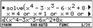 b. Press:
TI-89: [COPY]
TI-92 Plus: C
c. For this example, press ENTER to evaluate the entry.
 b. Press:
TI-89: [COPY]
TI-92 Plus: C
c. For this example, press ENTER to evaluate the entry.
Tip: You can also reuse an expression by creating a user-defined function. Refer to page 97.
- Paste the copied information into a new entry.
a. Press F3 1 to select the d differentiate function.
b. Press:
TI-89: [PASTE]
TI-92 Plus: V
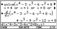 to paste the copied expression.
c. Complete the new entry, and press ENTER.
 to paste the copied expression.
c. Complete the new entry, and press ENTER.
Tip: By copying and pasting, you can easily transfer information from one application to another.
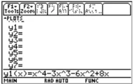
- Paste the copied information into a different application.
a. Press [Y=] to display the Y= Editor.
b. Press ENTER to define y1(x).
c. Press:
TI-89: [PASTE]
TI-92 Plus: V
 to paste.
d. Press ENTER to save the new definition.
 to paste.
d. Press ENTER to save the new definition.
96 Chapter 5: Additional Home Screen Topics
Creating and Evaluating User-Defined Functions
User-defined functions can be a great time-saver when you need to repeat the same expression (but with different values) multiple times. User-defined functions can also extend your TI-89 / TI-92 Plus's capabilities beyond the built-in functions.
Format of a Function
The following examples show user-defined functions with one argument and two arguments. You can use as many arguments as necessary. In these examples, the definition consists of a single expression (or statement).
Note: Function names follow the same rules as variable names. Refer to "Storing and Recalling Variable Values" in Chapter 2.
$ cube(x) = x^3 $ $ xroot(x,y) = y^1/x $
When defining functions and programs, use unique names for arguments that will not be used in the arguments for a subsequent function or program call.
In the argument list, be sure to use the same arguments that are used in the definition. For example, cube(n) = $x^3$ gives unexpected results when you evaluate the function.
Arguments (x and y in these examples) are placeholders that represent whatever values you pass to the function. They do not represent the variables x and y unless you specifically pass x and y as the arguments when you evaluate the function.
Creating a User-Defined Function
Use one of the following methods.


Creating a Multi-Statement Function
Note: For information about similarities and differences between functions and programs, refer to Chapter 17.
You can also create a user-defined function whose definition consists of multiple statements. The definition can include many of the control and decision-making structures (If, ElseIf, Return, etc.) used in programming.
For example, suppose you want to create a function that sums a series of reciprocals based on an entered integer (n):
$ 1/n + 1/n-1 + \dots + 1/1 $
When creating the definition of a multi-statement function, it may be helpful to visualize it first in a block form.
Variables not in the argument list must be declared as local. Returns a message if nn is not an integer or if nn≤0. Sums the reciprocals. Returns the sum.
Func Local temp,i If fPart(nn)≠0 or nn≤0 Return "bad argument" 0→temp For i,nn,1,-1 approx(temp+1/i)→temp EndFor Return temp EndFunc
Func and EndFunc must begin and end the function.
For information about the individual statements, refer to Appendix A.
When entering a multi-statement function on the Home screen, you must enter the entire function on a single line. Use the Define command just as you would for a single-statement function.
Use argument names that will never be used when calling the function or program. Use a colon to separate each statement.
Define sumrecip(nn)=Func:Local temp,i: ... :EndFunc
Tip: It's easier to create a complicated multi-statement function in the Program Editor than on the Home screen. Refer to Chapter 17.
On the Home screen:
Multi-statement functions show as "Func".
Enter a multi-statement function on one line. Be sure to include colons.

Evaluating a Function
You can use a user-defined function just as you would any other function. Evaluate it by itself or include it in another expression.

98 Chapter 5: Additional Home Screen Topics


Displaying and Editing a Function Definition
| To: | Do this: |
|---|---|
| Display a list of all user-defined functions | Press [2nd] [VAR-LINK] to display the VAR-LINK screen. You may need to use the [F2] View toolbar menu to specify the Function variable type. (Refer to Chapter 21.)— or —Press:TI-89: [CATALOG] [F4]TI-92 Plus: [2nd] [CATALOG] [F4] |
| Display a list of Flash application functions | Press:TI-89: [CATALOG] [F3]TI-92 Plus: [2nd] [CATALOG] [F3] |
| Display the definition of a user-defined function | From the VAR-LINK screen, highlight the function and display the Contents menu.TI-89: [2nd] [F6]TI-92 Plus: [F6]— or —From the Home screen, press [2nd] [RCL]. Type the function name but not the argument list (such as xroot), and press [ENTER] twice.— or —From the Program Editor, open the function. (Refer to Chapter 17.) |
| Edit the definition | From the Home screen, use [2nd] [RCL] to display the definition. Edit the definition as necessary. Then use [STO▶] or Define to save the new definition.— or —From the Program Editor, open the function, edit it, and save your changes. (Refer to Chapter 17.) |
Note: You can view a user-defined function in the CATALOG dialog box, but you cannot use the CATALOG to view or edit its definition.
Chapter 5: Additional Home Screen Topics 99
Using Folders to Store Independent Sets of Variables
The TI-89 / TI-92 Plus has one built-in folder named MAIN, and all variables are stored in that folder. By creating additional folders, you can store independent sets of user-defined variables (including user-defined functions).
Folders and Variables
Folders give you a convenient way to manage variables by organizing them into related groups. For example, you can create separate folders for different TI-89 / TI-92 Plus applications (Math, Text Editor, etc.) or classes.
- You can store a user-defined variable in any existing folder.
- A system variable or a variable with a reserved name, however, can be stored in the MAIN folder only.
Example of variables that can be stored in MAIN only
Window variables (xmin, xmax, etc.) Table setup variables (TblStart, \DeltaTbl, etc.) Y= Editor functions (y1(x), etc.)
The user-defined variables in one folder are independent of the variables in any other folder.
Therefore, folders can store separate sets of variables with the same names but different values.
Note: User-defined variables are stored in the "current folder" unless you specify otherwise. Refer to "Using Variables in Different Folders" on page 102.

Name of current folder
You cannot create a folder within another folder.
The system variables in the MAIN folder are always directly accessible, regardless of the current folder.
100 Chapter 5: Additional Home Screen Topics
Creating a Folder from the Home Screen
Enter the NewFold command.
NewFold folderName
Folder name to create. This new folder is set automatically as the current folder.
Creating a Folder from the VAR-LINK Screen
The VAR-LINK screen, which is described in Chapter 21, lists the existing variables and folders.
- Press 2nd [VAR-LINK].
- Press F1 Manage and select 5:Create Folder.
- Type a unique folder name up to eight characters, and press ENTER twice.
After you create a new folder from VAR-LINK, that folder is not automatically set as the current folder.
Setting the Current Folder from the Home Screen
Enter the setFold function.
setFold (folderName)
setFold is a function, which requires you to enclose the folder name in parentheses.
When you execute setFold, it returns the name of the folder that was previously set as the current folder.
Setting the Current Folder from the MODE Dialog Box
To use the MODE dialog box:
- Press MODE.
- Highlight the Current Folder setting.
- Press \text\textcircledD to display a menu of existing folders.
- Select the applicable folder. Either:
- Highlight the folder name and press ENTER. — or —
- Press the corresponding number or letter for that folder.
- Press ENTER to save your changes and close the dialog box.
Tip: To cancel the menu or exit the dialog box without saving any changes, press ESC.
Chapter 5: Additional Home Screen Topics 101


Using Variables in Different Folders
You can access a user-defined variable or function that is not in the current folder. Specify the complete pathname instead of only the variable name.
A pathname has the form: folderName\variableName — or — folderName\functionName
For example:
Note: This example assumes that you have already created a folder named MATH.
\begin{tabular}{|l|l|} \hline If Current Folder = MAIN & Folders \ \hline ■ 1 \rightarrow a \quad 1 & MAIN \ ■ $x^3 + x^2 + x + f(x)$ \quad Done & a=1 \ ■ 42 \rightarrow math\a \quad 42 & $f(x)=x^3+x^2+x$ \ ■ 3 \cdot x^2 + 4 \cdot x + 25 \rightarrow math\f(x) \quad Done & \ \multicolumn{1}{|l|}{3x^\wedge2+4x+25 \rightarrow math\f(x)} & \ \multicolumn{1}{|l|}{MAIN \quad RAD AUTO \quad FUNC \quad 4/30} & \ \hline ■ 4 \cdot a \quad 4 & MATH \ ■ 4 \cdot math\a \quad 168 & a=42 \ ■ f(5) \quad 155 & $f(x)=3x^2+4x+25$ \ ■ math\f(5) \quad 120 & \ \multicolumn{1}{|l|}{math\f(5)} & \ \multicolumn{1}{|l|}{MAIN \quad RAD AUTO \quad FUNC \quad 4/30} & \ \hline \end{tabular}
Note: For information about the VAR-LINK screen, refer to Chapter 21.
To see a list of existing folders and variables, press \boxed2nd [VAR-LINK]. On the VAR-LINK screen, you can highlight a variable and press \boxedENTER to paste that variable name to the Home screen's entry line. If you paste a variable name that is not in the current folder, the pathname (folderNamevariableName) is pasted.
Deleting a Folder from the Home Screen
Before deleting a folder, you must delete all the variables stored in that folder.
- To delete a variable, enter the DelVar command. DelVar var1 [, var2] [, var3] ...
Note: You cannot delete the MAIN folder.
- To delete an empty folder, enter the DelFold command. DelFold folder1 [, folder2] [, folder3] ...
Deleting a Folder from the VAR-LINK Screen
VAR-LINK lets you delete a folder and its variables at the same time. Refer to Chapter 21.
- Press \boxed2nd [VAR-LINK].
- Select the item(s) to delete and press \boxedF1 1 or \boxed\leftarrow. (If you use \boxedF4 to select a folder, its variables are selected automatically.)
- Press \boxedENTER to confirm the deletion.
102 Chapter 5: Additional Home Screen Topics

If an Entry or Answer Is “Too Big”
In some cases, an entry or answer may be “too long” and/or “too tall” to be displayed completely in the history area. In other cases, the TI-89 / TI-92 Plus may not be able to display an answer because there is not enough free memory.
If an Entry or Answer Is “Too Long”
Move the cursor into the history area, and highlight the entry or answer. Then use the cursor pad to scroll. For example:
- The following shows an answer that is too long for one line.
Press \blacklozenge or [2nd] \blacklozenge to scroll left.
 Press \blacklozenge or [2nd] \blacklozenge to scroll right.
- The following shows an answer that is both too long and too tall to be displayed on the screen.
TI-89: Press \blacktriangle or [T] \blacktriangle to scroll up. TI-92 Plus: Press \blacktriangle or [F4] \blacktriangle to scroll up
Note: This example uses the randMat function to generate a 25 x 25 matrix.
Press \blacklozenge or [2nd] \blacklozenge to scroll left.
 Press \blacklozenge or [2nd] \blacklozenge to scroll right.
TI-89: Press [T] \blacktriangledown to scroll down. TI-92 Plus: Press [F4] \blacktriangledown to scroll down
If There Is not Enough Memory
A $<<...>>$ symbol is displayed when the TI-89 / TI-92 Plus does not have enough free memory to display the answer.
For example:
Note: This example uses the seq function to generate a sequential list of integers from 1 to 2500.

When you see the $<<...>>$ symbol, the answer cannot be displayed even if you highlight it and try to scroll.
In general, you can try to:
- Free up additional memory by deleting unneeded variables and/or Flash applications. Use [2nd] [VAR-LINK] as described in Chapter 21.
- If possible, break the problem into smaller parts that can be calculated and displayed with less memory.
Chapter 5: Additional Home Screen Topics 103
104 Chapter 5: Additional Home Screen Topics
Basic Function Graphing
6
- Preview of Basic Function Graphing ........ 106
- Overview of Steps in Graphing Functions ........ 107
- Setting the Graph Mode ........ 108
- Defining Functions for Graphing ........ 109
- Selecting Functions to Graph ........ 111
- Setting the Display Style for a Function ........ 112
- Defining the Viewing Window ........ 113
- Changing the Graph Format ........ 114
- Graphing the Selected Functions ........ 115
- Displaying Coordinates with the Free-Moving Cursor ........ 116
- Tracing a Function ........ 117
- Using Zooms to Explore a Graph ........ 119
- Using Math Tools to Analyze Functions ........ 122
This chapter describes the steps used to display and explore a graph. Before using this chapter, you should be familiar with Chapter 2.

Y= Editor shows an algebraic representation.

Graph screen shows a graphic representation.
Although this chapter describes how to graph y(x) functions, the basic steps apply to all graphing modes. Later chapters give specific information about the other graphing modes.
Chapter 6: Basic Function Graphing 105
Preview of Basic Function Graphing
Graph a circle of radius 5, centered on the origin of the coordinate system. View the circle using the standard viewing window (ZoomStd). Then use ZoomSqr to adjust the viewing window.
| Steps | TI-89 Keystrokes | TI-92 Plus Keystrokes | Display |
|---|---|---|---|
| 1. Display the MODE dialog box. For Graph mode, select FUNCTION. | MODE► 1ENTER |
MODE► 1ENTER |
|
| 2. Display the Home screen. Then store the radius, 5, in variable r. | HOME5 STO► alpha RENTER |
♦ [HOME]5 STO► RENTER |
5►r |
| 3. Display and clear the Y= Editor. Then define y1(x) = √(r² - x²), the top half of a circle.In function graphing, you must define separate functions for the top and bottom halves of a circle. | ♦ [Y=]F1 8 ENTERENTER 2nd [√]alpha R ^ 2 - X^ 2 ) ENTER |
♦ [Y=]F1 8 ENTERENTER 2nd [√]R ^ 2 - X^ 2 ) ENTER |
|
| 4. Define y2(x) = -√(r² - x²), the function for the bottom half of the circle.The bottom half is the negative of the top half, so you can define y2(x) = -y1(x). | ENTER(-) Y 1 ( X )ENTER |
ENTER(-) Y 1 ( X )ENTER |
|
| 5. Select the ZoomStd viewing window, which automatically graphs the functions.In the standard viewing window, both the x and y axes range from -10 to 10. However, this range is spread over a longer distance along the x axis than the y axis. Therefore, the circle appears as an ellipse. | F2 6 |
F2 6 |
|
| 6. Select ZoomSqr.ZoomSqr increases the range along the x axis so that circles and squares are shown in correct proportion. | F2 5 |
F2 5 |
Note: There is a gap between the top and bottom halves of the circle because each half is a separate function. The mathematical endpoints of each half are (-5,0) and (5,0). Depending on the viewing window, however, the plotted endpoints for each half may be slightly different from their mathematical endpoints.
106 Chapter 6: Basic Function Graphing

Overview of Steps in Graphing Functions
To graph one or more y(x) functions, use the general steps shown below. For a detailed description of each step, refer to the following pages. You may not need to do all the steps each time you graph a function.
Graphing Functions
Tip: To turn off any stat data plots (Chapter 16), press [F5] 5 or use [F4] to deselect them.
Set Graph mode ([MODE]) to FUNCTION. Also set Angle mode, if necessary.
Define functions on Y= Editor ([\blacklozenge] [Y=]).
Select ([F4]) which defined functions to graph.

Tip: This is optional. For multiple functions, this helps visually distinguish one from another.
Set the display style for a function. TI-89: [2nd] [F6] TI-92 Plus: [F6]
Tip: [F2] Zoom also changes the viewing window.
Define the viewing window ([\blacklozenge] [WINDOW]).
Change the graph format, if necessary. [F1] 9 — or — TI-89: [\blacklozenge] [1] TI-92 Plus: [\blacklozenge] F
Graph the selected functions ([\blacklozenge] [GRAPH]).
Exploring the Graph
From the Graph screen, you can:
- Display the coordinates of any pixel by using the free-moving cursor, or of a plotted point by tracing a function.
- Use the [F2] Zoom toolbar menu to zoom in or out on a portion of the graph.
- Use the [F5] Math toolbar menu to find a zero, minimum, maximum, etc.
Chapter 6: Basic Function Graphing 107
Setting the Graph Mode
Before graphing y(x) functions, you must select FUNCTION graphing. You may also need to set the Angle mode, which affects how the TI-89 / TI-92 Plus graphs trigonometric functions.
Graph Mode
- Press
MODEto display the MODE dialog box, which shows the current mode settings. - Set the Graph mode to FUNCTION. Refer to “Setting Modes” in Chapter 2.
Note: For graphs that do not use complex numbers, set Complex Format = REAL. Otherwise, it may affect graphs that use powers, such as x^(1/3).

While this chapter specifically describes y(x) function graphs, the TI-89 / TI-92 Plus lets you select from six Graph mode settings.
| Graph Mode Setting | Description |
|---|---|
| FUNCTION | y(x) functions |
| PARAMETRIC | x(t) and y(t) parametric equations |
| POLAR | r(θ) polar equations |
| SEQUENCE | u(n) sequences |
| 3D | z(x,y) 3D equations |
| DIFFERENTIAL EQUATION | y'(t) differential equations |
Note: Other Graph mode settings are described in later chapters.
Angle Mode
When using trigonometric functions, set the Angle mode for the units (RADIAN or DEGREE) in which you want to enter and display angle values.
Checking the Status Line
To see the current Graph mode and Angle mode, check the status line at the bottom of the screen.
108 Chapter 6: Basic Function Graphing