Setting the Initial Conditions
You can enter initial conditions in the Y= Editor, let the TI-89 / TI-92 Plus calculate initial conditions automatically, or select them interactively from the Graph screen.
Entering Initial Conditions in the Y= Editor
You can specify one or more initial conditions in the Y= Editor. To specify more than one, enter them as a list enclosed in braces { } and separated by commas.
To enter initial conditions for the y1' equation, use the y1 line, etc.
To specify when the initial conditions occur, use t0. This is also the first t evaluated for the graph.
To graph a family of solutions, enter a list of initial conditions.
Enter {10,20} even though {10 20} is displayed.
Note: For information about defining a system for higher-order equations, refer to page 186.
For a 2nd- or higher-order differential equation, you must define a system of 1st-order equations in the Y= Editor.
If you enter initial conditions, you must enter the same number of initial conditions for each equation in the system. Otherwise, a Dimension error occurs.
If You Do Not Enter an Initial Condition in the Y= Editor
If you do not enter initial conditions, the ncurves Window variable (□[WINDOW]) specifies the number of solution curves graphed automatically. By default, ncurves = 0. You can enter a value from 0 through 10. However, the Fields graph format and the Axes setting determine whether ncurves is used.
Tip: Without entering initial conditions, use SLPFLD (with ncurves=0) or DIRFLD to display a slope or direction field only.
Note: SLPFLD is for a single 1st-order equation only. DIRFLD is for a 2nd-order equation (or system of two 1st-order equations) only.
| If Fields = | Then: |
|---|---|
| SLPFLD | Uses ncurves, if not set to 0, to graph curves. |
| DIRFLD | Ignores ncurves. Does not graph any curves. |
| FLDOFF | Uses ncurves if Axes = TIME (or if Axes = Custom and the x axis is t). Otherwise, a Diff Eq setup error occurs. |
When ncurves is used, t0 is set temporarily at the middle of the Graph screen. However, the value of t0 as set in the Y= Editor or Window Editor is not changed.
184 Chapter 11: Differential Equation Graphing


Selecting an Initial Condition Interactively from the Graph Screen
Note: With SLPFLD or DIRFLD, you can select initial conditions interactively regardless of whether you enter initial conditions in the Y= Editor.
When a differential equation is graphed (regardless of whether a solution curve is displayed), you can select a point on the Graph screen and use it as an initial condition.
Note about Tracing a Solution Curve
When you enter initial conditions in the Y= Editor or let ncurves graph solution curves automatically, you can use F3 to trace the curves.
However, you cannot trace a curve drawn by selecting an initial condition interactively. These curves are drawn, not plotted.
Chapter 11: Differential Equation Graphing 185


Defining a System for Higher-Order Equations
In the Y= Editor, you must enter all differential equations as 1st-order equations. If you have an $n^{th}$-order equation, you must transform it into a system of $n$ 1st-order equations.
Transforming an Equation into a 1st-Order System
A system of equations can be defined in various ways, but the following is a general method.
- Rewrite the original differential equation as necessary. a. Solve for the highest-ordered derivative. b. Express it in terms of y and t. c. On the right side of the equation only, substitute to eliminate any references to derivative values.
Note: To produce a 1st-order equation, the right side must contain non-derivative variables only.
\begin{tabular}{ll} In place of: & Substitute: \ y & y1 \ y' & y2 \ y'' & y3 \ y''' & y4 \ y$^{(4)}$ & y5 \ \vdots & \vdots \ \end{tabular}
d. On the left side of the equation, substitute for the derivative value as shown below.
\begin{tabular}{ll} In place of: & Substitute: \ y' & y1' \ y'' & y2' \ y''' & y3' \ y$^{(4)}$ & y4' \ \vdots & \vdots \ \end{tabular}
Note: Based on the above substitutions, the y' lines in the Y= Editor represent: y1' = y' y2' = y'' etc. So, this example's 2nd-order equation is entered on the y2' line.
- On the applicable lines in the Y= Editor, define the system of equations as: y1' = y2 y2' = y3 y3' = y4 – up to – yn' = your $n^{th}$-order equation
In a system such as this, the solution to the y1' equation is the solution to the $n^{th}$-order equation. You may want to deselect any other equations in the system.
186 Chapter 11: Differential Equation Graphing

Example of a 2nd-Order Equation
The 2nd-order differential equation y''+y = 0 represents a simple harmonic oscillator. Transform this into a system of equations for the Y= Editor. Then, graph the solution for initial conditions y(0) = 0 and y'(0) = 1.
Example
-
Press [MODE] and set Graph=DIFF EQUATIONS.
-
Define a system of equations for the 2nd-order equation as described on page 186. Rewrite the equation and make the necessary substitutions.
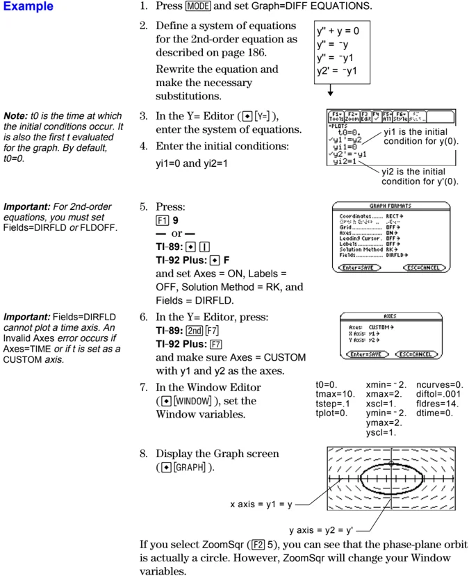 Note: t0 is the time at which the initial conditions occur. It is also the first t evaluated for the graph. By default, t0=0.
-
In the Y= Editor (□[Y=]), enter the system of equations.
-
Enter the initial conditions: yi1=0 and yi2=1
yi1 is the initial condition for y(0). yi2 is the initial condition for y'(0).
 Note: t0 is the time at which the initial conditions occur. It is also the first t evaluated for the graph. By default, t0=0.
Important: For 2nd-order equations, you must set Fields=DIRFLD or FLDOFF. 5. Press: F1 9 — or — TI-89: □ [1] TI-92 Plus: □ F and set Axes = ON, Labels = OFF, Solution Method = RK, and Fields = DIRFLD.
Important: Fields=DIRFLD cannot plot a time axis. An Invalid Axes error occurs if Axes=TIME or if t is set as a CUSTOM axis. 6. In the Y= Editor, press: TI-89: [2nd] [F7] TI-92 Plus: [F7] and make sure Axes = CUSTOM with y1 and y2 as the axes.
-
In the Window Editor ([□[WINDOW]]), set the Window variables. t0=0. xmin=-2. ncurves=0. tmax=10. xmax=2. diftol=.001 tstep=1 xscl=1. fldres=14. tplot=0. ymin=-2. dtime=0. ymax=2. yscl=1.
-
Display the Graph screen ([□[GRAPH]]).
x axis = y1 = y y axis = y2 = y'
If you select ZoomSqr ([F2] 5), you can see that the phase-plane orbit is actually a circle. However, ZoomSqr will change your Window variables.
Chapter 11: Differential Equation Graphing 187
To examine this harmonic oscillator in more detail, use a split screen to graph the manner in which y and y' change with respect to time (t).
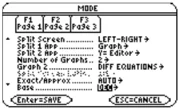
Note: To display different graphs in both parts of a split screen, you must use the 2-graph mode.
-
Press MODE and change the mode settings on Page 2 as shown. Then close the MODE dialog box, which redraws the graph.
-
Press 2nd [box with right arrow] to switch to the right side of the split screen.
-
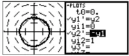
Use F4 to select y1' and y2'. The right side uses the same equations as the left side. However, no equations are selected initially in the right side.
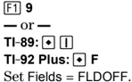
Important: Because Fields=DIRFLD cannot plot a time axis, you must change the Fields setting. FLDOFF turns off all fields.
-
Press: F1 9 — or — TI-89: [box with dot] [box with I] TI-92 Plus: [box with dot] F Set Fields = FLDOFF.
-
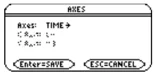
In the Y= Editor, press: TI-89: 2nd F7 TI-92 Plus: F7 and make sure Axes = TIME.
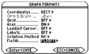
Note: When you enter 2-graph mode, Window variables for the right side are set to their defaults.
-
In the Window Editor, change ymin and ymax as shown to the right. ymin=-2. ymax=2.
-
Press [box with dot] [GRAPH] to display the Graph screen for graph #2. The left side shows the phase-plane orbit. The right side shows the solution curve and its derivative.
 y' y
-
To return to a full screen of the original graph, press 2nd [box with right arrow] to switch to the left side. Then press MODE and change the Split Screen setting. Split Screen = FULL
 y' y
188 Chapter 11: Differential Equation Graphing

Example of a 3rd-Order Equation
For the 3rd-order differential equation y''' + 2y'' + 2y' + y = sin(x), write a system of equations to enter in the Y= Editor. Then graph the solution as a function of time. Use initial conditions y(0) = 0, y'(0) = 1, and y''(0) = 1.
Example
- Press MODE and set Graph=DIFF EQUATIONS.
- Define a system of equations for the 3rd-order equation as described on page 186.
Rewrite the equation and make the necessary substitutions.
$$ \begin{aligned} &y''' + 2y'' + 2y' + y = \sin(x) \ &y''' = \sin(x) - 2y'' - 2y' - y \ &y''' = \sin(t) - 2y'' - 2y' - y \ &y''' = \sin(t) - 2y3 - 2y2 - y1 \ &y3' = \sin(t) - 2y3 - 2y2 - y1 \end{aligned} $$
Note: t0 is the time at which the initial conditions occur. By default, t0=0.
- In the Y= Editor ( [Y=] ), enter the system of equations.
- Enter the initial conditions: yi1=0, yi2=1, and yi3=1

Important: The solution to the y1' equation is the solution to the 3rd-order equation.
- Be sure that only y1' is selected. Use F4 to deselect any other equations.
Important: For 3rd- or higher-order equations, you must set Fields=FLDOFF. Otherwise, an Undefined variable error occurs when graphing.
- Press: F1 9 — or — TI-89: [F] TI-92 Plus: [F] F Set Axes = ON, Labels = ON, Solution Method = RK, and Fields = FLDOFF.
Note: With Axes=TIME, the solution to the selected equation is plotted against time (t).
-
In the Y= Editor, press: TI-89: [2nd] [F7] TI-92 Plus: [F7] Set Axes = TIME.
-
In the Window Editor ([WINDOW]), set the Window variables.
t0=0. xmin=-1. ncurves=0. tmax=10. xmax=10. diftol=.001 tstep=.1 xscl=1. tplot=0. ymin=-3. ymax=3. yscl=1.
Tip: To find the solution at a particular time, use [F3] to trace the graph.
- Display the Graph screen ([GRAPH]).
Chapter 11: Differential Equation Graphing 189


Setting Axes for Time or Custom Plots
Setting the axes can give you great flexibility in graphing differential equations. Custom axes are particularly effective for showing different kinds of relationships.
Displaying the AXES Dialog Box
From the Y= Editor, press:
- TI-89: [2nd] [F7]
- TI-92 Plus: [F7]

If Fields = SLPFLD, Axes is unavailable.
- TI-89: [2nd] [F7]
- TI-92 Plus: [F7]
| Item | Description |
|---|---|
| Axes | TIME — Plots t on the x axis and y (solutions to all selected differential equations) on the y axis.CUSTOM — Lets you select the x and y axes. |
| X Axis, Y Axis | Active only when Axes = CUSTOM, these let you select what you want to plot on the x and y axes. |

Note: t is not valid for either Axis when Fields=DIRFLD. If you select t, an Invalid axes error occurs when graphing.
- t — time
- y — solutions (y1, y2, etc.) of all selected differential equations
- y' — values of all selected differential equations (y1', y2', etc.)
- y1, y2, etc. — the solution to the corresponding differential equation, regardless of whether that equation is selected
- y1', y2', etc. — the value of the right-hand side of the corresponding differential equation, regardless of whether that equation is selected
190 Chapter 11: Differential Equation Graphing
Example of Time and Custom Axes
Using the predator-prey model from biology, determine the numbers of rabbits and foxes that maintain population equilibrium in a certain region. Graph the solution using both time and custom axes.
Predator-Prey Model
Use the two coupled 1st-order differential equations:
$y1' = -y1 + 0.1y1 * y2$ and $y2' = 3y2 - y1 * y2$
where:
$y1$ = Population of foxes $yi1$ = Initial population of foxes (2) $y2$ = Population of rabbits $yi2$ = Initial population of rabbits (5)
Tip: To speed up graphing times, clear any other equations in the Y= Editor. With FLDOFF, all equations are evaluated even if they are not selected.
-
Use [MODE] to set Graph = DIFF EQUATIONS.
-
In the Y= Editor ([♦][Y=]), define the differential equations and enter the initial conditions.
-
Press: [F1] 9 — or — TI-89: [♦] [1] TI-92 Plus: [♦] F Set Axes = ON, Labels = ON, Solution Method = RK, and Fields = FLDOFF.
-
In the Y= Editor, press: TI-89: [2nd] [F7] TI-92 Plus: [F7] Set Axes = TIME.
-
In the Window Editor ([♦][WINDOW]), set the Window variables.
$t0=0.$ $tmax=10.$ tstep=\pi/24 $tplot=0.$ $xmin=-1.$ $xmax=10.$ $xscl=5.$ $ymin=-10.$ $ymax=40.$ $yscl=5.$ $ncurves=0.$ $diftol=.001$
-
Graph the differential equations ([♦][GRAPH]).
-
Press [F3] to trace. Then press 3 [ENTER] to see the number of foxes (yc for y1) and rabbits (yc for y2) at t=3.
Tip: Use [⊕] and [⊖] to move the trace cursor between the curves for y1 and y2.

Chapter 11: Differential Equation Graphing 191


Note: In this example, DIRFLD is used for two related differential equations that do not represent a 2nd-order equation.
-
Return to the Y= Editor. Press: F1 9 — or — TI-89: [♦] [F1] TI-92 Plus: [♦] F Set Fields = DIRFLD.
-
Press: TI-89: [2nd] [F7] TI-92 Plus: [F7] Confirm that the axes are set as shown.
-
In the Y= Editor, clear the initial conditions for yi1 and yi2.
-
Return to the Graph screen, which displays only the direction field.
Tip: Use a list to specify more than one initial condition.
-
To graph a family of solutions, return to the Y= Editor and enter the initial conditions shown below. yi1={2,6,7} and yi2={5,12,18}
-
Return to the Graph screen, which displays a curve for each pair of initial conditions.
Tip: Use [◄] and [►] to move the trace cursor from one initial condition curve to another.
- Press [F3] to trace. Then press 3 [ENTER] to see the number of foxes (xc) and rabbits (yc) at t=3. Because t0=0 and tmax=10, you can trace in the range 0≤t≤10.
192 Chapter 11: Differential Equation Graphing

Example Comparison of RK and Euler
Consider a logistic growth model dP/dt = .001 * P * (100 – P), with the initial condition P(0) = 10. Use the BldData instruction to compare the graphing points calculated by the RK and Euler solution methods. Then plot those points along with a graph of the equation’s exact solution.
Example
-
Press MODE and set Graph=DIFF EQUATIONS.
-
Express the 1st-order equation in terms of y1' and y1. y1'= .001y1*(100-y1)
Do not use implied multiplication between the variable and parentheses. If you do, it is treated as a function call.
Tip: To speed up graphing times, clear any other equations in the Y= Editor. With FLDOFF, all equations are evaluated even if they are not selected.
- Enter the equation in the Y= Editor ( [Y=] ).
- Enter the initial condition: yi1=10
 t0 is the time at which the initial condition occurs. By default, t0=0.
-
Press: F1 9 — or — TI-89: [F1] TI-92 Plus: [F] F Set Solution Method = RK and Fields = FLDOFF.
-
In the Window Editor ([WINDOW]), set the Window variables.
t0=0. xmin=-1. ncurves=0. tmax=100. xmax=100. diftol=.001 tstep=1. xscl=1. tplot=0. ymin=-10. ymax=10. yscl=1.
Important: Change tstep from .1 (its default) to 1. Otherwise, BldData calculates too many rows for the data variable and a Dimension error occurs.
Note: You do not need to graph the equation before using BldData. For more information about BldData, refer to Appendix A.
-
In the Home screen TI-89: [HOME] TI-92 Plus: [HOME] use BldData to create a data variable containing the RK graphing points.
BldData rklog
-
Return to the Y= Editor, press: F1 9 — or — TI-89: [F1] TI-92 Plus: [F] F Set Solution Method = EULER.
Chapter 11: Differential Equation Graphing 193
- Return to the Home screen, and use BldData to create a data variable containing the Euler graphing points.
Note: errorlog lets you combine the data in rklog and eulerlog so that you can view the two sets of data side by side.
Note: rklog[1] and rklog[2] refer to column 1 and 2 in rklog, respectively. Likewise with eulerlog[2].
Tip: Scroll through the data variable to see how the RK and Euler values differ for the same time value.
-
Use the Data/Matrix Editor (APPS 6 3) to create a new data variable named errorlog.
-
In this new data variable, define the c1, c2, and c3 column headers to refer to data in rklog and eulerlog. Also, enter column titles as shown.
To define a column header, move the cursor to that column, press F4, type the reference expression (such as rklog[1] for c1), and press ENTER.
-
In the Data/Matrix Editor, press F2. Then press F1 and define Plot 1 for the RK data, as shown to the right.
-
Define Plot 2 for the Euler data. Use the values shown to the right.
-
Return to the Y= Editor, press MODE, and set Graph = FUNCTION.
Note: To see how to use deSolve() to find this exact, general solution, refer to page 196.
- The exact solution to the differential equation is given below. Enter it as y1.
$$y1 = (100* e^{(x/10)})/(e^{(x/10)}+9)$$

Plot Type=xyl ine Mark=Cross x=c1 y=c3
You can use \odot to scroll up to see Plot 1 and Plot 2.
194 Chapter 11: Differential Equation Graphing


- In the Window Editor, set the Window variables.
Note: The fuzzy line on the graph indicates differences between the RK and Euler values.
- Display the Graph screen ( [icon] [GRAPH] ).
xmin= -10. ymin= -10. xres=2. xmax=100. ymax=120. xscl=10. yscl=10.
- In the Window Editor, set the Window variables to zoom in so that you can examine the differences in more detail.
xmin=39.7 ymin=85.5 xres=2. xmax=40.3 ymax=86. xscl=.1 yscl=.1
-
Return to the Graph screen.
-
Press F3 to trace, and then press \odot or \odot until y1 is selected. (1 shows in upper right corner.) Then enter 40.
y1 is selected when 1 shows here. —
By moving the trace cursor to trace each solution to xc = 40, you can find that:
- The exact solution (y1) is 85.8486, rounded to six digits.
- The RK solution (Plot 1) is 85.8952.
- The Euler solution (Plot 2) is 85.6527.
You can also use the Data/Matrix Editor to open the errorlog data variable and scroll to time = 40.
Chapter 11: Differential Equation Graphing 195

Example of the deSolve() Function
The deSolve() function lets you solve many 1st- and 2nd-order ordinary differential equations exactly.
Example
For a general solution, use the following syntax. For a particular solution, refer to Appendix A.
deSolve(1stOr2ndOrderODE, independentVar, dependentVar)
Using the logistic 1st-order differential equation from the example on page 176, find the general solution for y with respect to t.
deSolve(y' = 1/1000 y* (100- y),t,y)
Tip: For maximum accuracy, use 1/1000 instead of .001. A floating-point number can introduce round-off errors.
Note: This example does not involve graphing, so you can use any Graph mode.
Do not use implied multiplication between the variable and parentheses. If you do, it will be treated as a function call.
For ', type [2nd] [·].
Before using deSolve(), clear any existing t and y variables. Otherwise, an error occurs.
- In the Home screen TI-89: [HOME] TI-92 Plus: [F4] [HOME] use deSolve() to find the general solution.

@1 represents a constant. You may get a different constant (@2, etc.).
- Use the solution to define a function. a. Press [◄►] to highlight the solution in the history area. Then press [ENTER] to autopaste it into the entry line. b. Insert the Define instruction at the beginning of the line. Then press [ENTER].
Tip: Press [2nd] [◄] to move to the beginning of the entry line.

- For an initial condition y=10 with t=0, use solve() to find the @1 constant.
Note: If you got a different constant (@2, etc.), solve for that constant.

For @, type TI-89: [2nd] [STO►] TI-92 Plus: [2nd] R
- Evaluate the general solution (y) with the constant @1=9/100 to obtain the particular solution shown.
You can also use deSolve() to solve this problem directly. Enter: deSolve(y' = 1/1000 y* (100- y) and y(0)=10,t,y)
196 Chapter 11: Differential Equation Graphing
Troubleshooting with the Fields Graph Format
If you have difficulties graphing a differential equation, this section can help you correct the problem. Many problems may be related to your Fields graph format setting.
Setting the Fields Graph Format
From the Y= Editor, Window Editor, or Graph screen, press:
F1 9
— or —
TI-89: □ 1
TI-92 Plus: □ F

What Order Equation Are You Graphing?
| If the equation is: | Valid Fields settings are: |
|---|---|
| 1st-order | SLPFLD or FLDOFF |
| 2nd-order (system of two 1st-order equations) | DIRFLD or FLDOFF |
| 3rd- or higher-order (system of three or more 1st-order equations) | FLDOFF |
Because Fields = SLPFLD is the default setting, a common error message is shown to the right.

When you see this or any other error message:
- For your order of equation, use the previous table to find the valid Fields settings. Change to the applicable setting.
- For a particular Fields setting, check the following for information that applies to that setting.
Fields=SLPFLD
| In the Y= Editor | Use F4 to select one and only one 1st-order equation. You can enter multiple equations, but only one at a time can be selected. The selected equation must not refer to any other equation in the Y= Editor. For example: If y1'=y2, an Undefined variable error occurs when you graph. |
|---|---|
| In the Graph screen | If the slope field is drawn but no solution curve is plotted, specify an initial condition as described on page 184. |

Chapter 11: Differential Equation Graphing 197
Fields=DIRFLD
In the Y= Editor
Enter a valid system of two 1st-order equations. For information about defining a valid system for a 2nd-order equation, refer to page 186.
Set Axes = CUSTOM:
- TI-89:
2nd[F7] - TI-92 Plus:
[F7]
If Axes = TIME, an Invalid axes error occurs when you graph.
If you enter initial conditions in the Y= Editor, the equations referenced by the custom axes must have the same number of initial conditions.
Otherwise, a Dimension error occurs when you graph.

With custom axes
Set axes that are valid for your system of equations.
Do not select t for either axis. Otherwise, an Invalid axes error occurs when you graph.
The two axes must refer to different equations in your system of equations. For example, y1 vs. y2 is valid, but y1 vs. y1' gives an Invalid axes error.
In the Graph screen
If the direction field is drawn but no curve is plotted, enter initial conditions in the Y= Editor or select one interactively from the Graph screen as described starting on page 184. If you did enter initial conditions, select ZoomFit:
- TI-89:
[F2][alpha]A - TI-92 Plus:
[F2]A
The ncurves Window variable is ignored with DIRFLD. Default curves are not drawn automatically.
Notes
With DIRFLD, the equations referenced by the custom axes determine which equations are graphed, regardless of which equations are selected in the Y= Editor.
If your system of equations refers to t, the direction field (not the plotted curves) is drawn with respect to one particular time, which is set by the dtime Window variable.
198 Chapter 11: Differential Equation Graphing

Fields=FLDOFF
In the Y= Editor
If you enter a 2nd- or higher-order equation, enter it as a valid system of equations as described on page 186.
All equations (selected or not) must have the same number of initial conditions. Otherwise, a Dimension error occurs when you graph.
To set Axes = TIME or CUSTOM, press:
- TI-89:
2nd[F7] - TI-92 Plus:
[F7]

With custom axes
If X Axis is not t, you must enter at least one initial condition for each equation in the Y= Editor (whether the equation is selected or not).
Otherwise, a Diff Eq setup error occurs when you graph.

In the Graph screen
If no curve is graphed, set an initial condition as described on page 184. If you did enter initial conditions in the Y= Editor, select ZoomFit:
- TI-89:
[F2][alpha]A - TI-92 Plus:
[F2]A
A 1st-order equation may look different with FLDOFF than with SLPFLD. This is because FLDOFF uses the tplot and tmax Window variables (page 181), which are ignored with SLPFLD.
Notes
For 1st-order equations, use FLDOFF and Axes = Custom to plot axes that are not possible with SLPFLD. For example, you can plot t vs. y1' (where SLPFLD plots t vs. y1). If you enter multiple 1st-order equations, you can plot one equation or its solution vs. another by specifying them as the axes.
If You Use the Table Screen to View Differential Equations
You can use the Table screen to view the points for a differential equation graph. However, the table may show different equations than those graphed. The table shows only the selected equations, regardless of whether those equations will be plotted with your current Fields and Axes settings.
Chapter 11: Differential Equation Graphing 199
200 Chapter 11: Differential Equation Graphing
Additional Graphing Topics
12
- Preview of Additional Graphing Topics ........ 202
- Collecting Data Points from a Graph ........ 203
- Graphing a Function Defined on the Home Screen ........ 204
- Graphing a Piecewise Defined Function ........ 206
- Graphing a Family of Curves ........ 208
- Using the Two-Graph Mode ........ 209
- Drawing a Function or Inverse on a Graph ........ 212
- Drawing a Line, Circle, or Text Label on a Graph ........ 213
- Saving and Opening a Picture of a Graph ........ 217
- Animating a Series of Graph Pictures ........ 219
- Saving and Opening a Graph Database ........ 220
This chapter describes additional features that you can use to create graphs on the TI-89 / TI-92 Plus. This information generally applies to all Graph mode settings.

This chapter assumes that you already know the fundamental procedures for defining and selecting functions, setting Window variables, and displaying graphs as described in Chapter 6: Basic Function Graphing.
Chapter 12: Additional Graphing Topics 201

Preview of Additional Graphing Topics
From the Home screen, graph the piecewise defined function: y = -x when x < 0 and y = 5 cos(x) when x ≥ 0. Draw a horizontal line across the top of the cosine curve. Then save a picture of the displayed graph.
| Steps | TI-89 Keystrokes | TI-92 Plus Keystrokes | Display |
|---|---|---|---|
| 1. Display the MODE dialog box. For Graph mode, select FUNCTION. For Angle mode, select RADIAN. | [MODE] ▸ 1 ▾ ▾ ▸ 1 [ENTER] | [MODE] ▸ 1 ▾ ▾ ▸ 1 [ENTER] | |
| 2. Display the Home screen. Use the Graph command and the when function to specify the piecewise defined function. [F4] 2 selects Graph from the Other toolbar menu and automatically adds a space. | [HOME] [F4] 2 [2nd] [a-lock] W H E N [alpha] ( ( X [2nd] [‹] 0 , (-) X , 5 × [2nd] [COS] X ) ) | ◆ [HOME] [F4] 2 W H E N ( ( X [2nd] [‹] 0 , (-) X , 5 × [COS] X ) ) | Graph when(x<0,-x,5*cos(x)) |
| 3. Execute the Graph command, which automatically displays the Graph screen. The graph uses the current Window variables, which are assumed to be their standard values ([F2] 6) for this example. | [ENTER] | [ENTER] | |
| 4. Draw a horizontal line across the top of the cosine curve. The calculator remains in “line” mode until you select a different operation or press [ESC]. | [2nd] [F7] 5 ◯ (until the line is positioned) [ENTER] | [F7] 5 ◯ (until the line is positioned) [ENTER] | |
| 5. Save a picture of the graph. Use PIC1 as the variable name for the picture. Be sure to set Type = Picture. By default, it is set to GDB. | [F1] 2 ▸ 2 ◯ ▸ P I C [alpha] 1 [ENTER] [ENTER] | [F1] 2 ▸ 2 ◯ ▸ P I C 1 [ENTER] [ENTER] | |
| 6. Clear the drawn horizontal line. You can also press [F4] to regraph. | [2nd] [F6] 1 | [F6] 1 | |
| 7. Open the saved picture variable to redisplay the graph with the line. Be sure to set Type = Picture. By default, it is set to GDB. | [F1] 1 ▸ 2 (if not already shown, also set Variable = pic1) [ENTER] | [F1] 1 ▸ 2 (if not already shown, also set Variable = pic1) [ENTER] |
202 Chapter 12: Additional Graphing Topics

Collecting Data Points from a Graph
From the Graph screen, you can store sets of coordinate values and/or math results for later analysis. You can store the information as a single-row matrix (vector) on the Home screen or as data points in a system data variable that can be opened in the Data/Matrix Editor.
Collecting the Points
- Display the graph. (This example shows y1(x)=5*cos(x).)
- Display the coordinates or math results you want to collect.
- Save the information to the Home screen or the sysData variable. TI-89: \blacklozenge \square (Home screen) or \blacklozenge \square (sysData variable) TI-92 Plus: \blacklozenge H (Home screen) or \blacklozenge D (sysData variable)
- Repeat the process as necessary.
Tip: To display coordinates or math results, trace a function with F3 or perform an F5 Math operation (such as Minimum or Maximum). You can also use the free-moving cursor.

TI-89: \blacklozenge \square TI-92 Plus: \blacklozenge H
\swarrow
Displayed coordinates are added to the Home screen's history area (but not the entry line) as a single-row matrix or vector.
\searrow
TI-89: \blacklozenge \square TI-92 Plus: \blacklozenge D
Displayed coordinates are stored in a data variable named sysData, which you can open in the Data/Matrix Editor.
Tip: Use a split screen to show a graph and the Home screen or Data/Matrix Editor at the same time.
Notes about SysData Variable
- When you press: TI-89: \blacklozenge \square TI-92 Plus: \blacklozenge D
- If sysData does not exist, it is created in the MAIN folder.
- If sysData already exists, new data is appended to the end of any existing data. Existing titles or column headers (for the affected columns) are cleared; titles are replaced with the applicable titles for the new data.
- The sysData variable can be cleared, deleted, etc., just as any other data variable. However, it cannot be locked.
- If the Graph screen contains a function or stat plot that references the current contents of sysData, this command will not operate.
Chapter 12: Additional Graphing Topics 203
Graphing a Function Defined on the Home Screen
In many cases, you may create a function or expression on the Home screen and then decide to graph it. You can copy an expression to the Y= Editor, or graph it directly from the Home screen without using the Y= Editor.
What Is the "Native" Independent Variable?
On the Y= Editor, all functions must be defined in terms of the current graph mode's "native" independent variable.
Copying from the Home Screen to the Y= Editor
If you have an expression on the Home screen, you can use any of the following methods to copy it to the Y= Editor.
Tip: Instead of using F1 5 or F1 6 to copy and paste, use:
TI-89: [COPY] or [PASTE]. TI-92 Plus: C (copy) or V(paste).
Tip: To copy an expression from the Home screen's history area to the entry line, use the auto-paste feature or copy and paste.
Tip: Define is available from the Home screen's F4 toolbar menu.
Tip: 2nd RCL is useful if an expression is stored to a variable or function that does not correspond to the Y= Editor, such as a1 or f1(x).
204 Chapter 12: Additional Graphing Topics

Graphing Directly from the Home Screen
The Graph command lets you graph an expression from the Home screen without using the Y= Editor. Unlike the Y= Editor, Graph lets you specify an expression in terms of any independent variable, regardless of the current graphing mode.
Tip: Graph is available from the Home screen’s F4 toolbar menu.
Note: Graph uses the current Window variable settings.
\begin{tabular}{|l|l|} \hline If the expression is in terms of: & Use the Graph command as shown in this example: \ \hline The native independent variable & \texttt{graph 1.25xcos(x)} \ & For function graphing, \sqcup x is the native variable. \ \hline A non-native independent variable & \texttt{graph 1.25acos(a),a} \ & Specify the independent variable; otherwise, you may get an error. \ \hline \end{tabular}
Tip: To create a table from the Home screen, use the Table command. It is similar to Graph. Both share the same expressions.
Graph does not work with sequence graphs or differential equations. For parametric, polar, and 3D graphs, use the following variations.
In PARAMETRIC graphing mode: \quad Graph xExpr, yExpr, t In POLAR graphing mode: \qquad\qquad Graph expr, \theta In 3D graphing mode: \qquad\qquad\quad Graph expr, x, y
Graph does not copy the expression to the Y= Editor. Instead, it temporarily suspends any functions selected on the Y= Editor. You can trace, zoom, or show and edit Graph expressions on the Table screen, just the same as Y= Editor functions.
Clearing the Graph Screen
Each time you execute Graph, the new expression is added to the existing ones. To clear the graphs:
- Execute the ClrGraph command (available from the Home screen’s F4 Other toolbar menu). — or —
- Display the Y= Editor. The next time you display the Graph screen, it will use the functions selected on the Y= Editor.
Extra Benefits of User-Defined Functions
You can define a user-defined function in terms of any independent variable. For example:
Defined in terms of "aa". define f1(aa)=1.25aa*cos(aa) graph f1(x)
and: Refers to the function by using the native independent variable. define f1(aa)=1.25aa*cos(aa) f1(x)→y1(x)
Chapter 12: Additional Graphing Topics 205

Graphing a Piecewise Defined Function
To graph a piecewise function, you must first define the function by specifying boundaries and expressions for each piece. The when function is extremely useful for two-piece functions. For three or more pieces, it may be easier to create a multi-statement, user-defined function.
Using the When Function
Tip: Graph math results may vary.
To define a two-piece function, use the syntax:
when(condition, trueExpression, falseExpression)
For example, suppose you want to graph a function with two pieces.
| When: | Use expression: |
|---|---|
| x < 0 | -x |
| x ≥ 0 | 5 cos(x) |

In the Y= Editor:
The function is pretty printed in this form.
Enter the function in this form.

Tip: To enter when, type it or use the CATALOG.
For three or more pieces, you can use nested when functions.
| When: | Use expression: |
|---|---|
| x < -π | 4 sin(x) |
| x ≥ -π and x < 0 | 2x + 6 |
| x ≥ 0 | 6 -x² |

In the Y= Editor:
where:
y1(x)=when(x<0,when(x<-π,4*sin(x),2x+6),6-x^2)
This nested function is in effect when x<0.
Nested functions quickly become complex and difficult to visualize.
206 Chapter 12: Additional Graphing Topics
Using a Multi-Statement, User-Defined Function
For three or more pieces, you may want to create a multi-statement, user-defined function.
For example, consider the previous three-piece function.

Note: For information about similarities and differences between functions and programs, refer to Chapter 17.
Tip: Graph math results may vary.
A multi-statement, user-defined function can have many of the control and decision-making structures (If, ElseIf, Return, etc.) used in programming. When creating the structure of a function, it may be helpful to visualize it first in a block form.
Func If x< -π Then Return 4*sin(x) ElseIf x>=-π and x<0 Then Return 2x+6 Else Return 6-x^2 EndIf EndFunc
Func and EndFunc must begin and end the function.
For information about the individual statements, refer to Appendix A.
When entering a multi-statement function on the Y= Editor or Home screen, you must enter the entire function on a single line.
Use a colon (:) to separate each statement.
Func:If x< -π Then:Return 4*sin(x): ... :EndIf:EndFunc
On the Y= Editor:
Only "Func" is shown for a multi-statement function.
Enter a multi-statement function on one line. Be sure to include colons.

From the Home Screen or a Program
From the Home screen, you can also use the Define command to create a multi-statement, user-defined function. Refer to page 204 for other information on copying a function from the Home screen to the Y= Editor.
From the Program Editor (Chapter 17), you can create a user-defined function. For example, use the Program Editor to create a function named f1(xx). In the Y= Editor, set y1(x) = f1(x).


Graphing a Family of Curves
By entering a list in an expression, you can plot a separate function for each value in the list. (You cannot graph a family of curves in SEQUENCE or 3D graphing mode.)
Examples Using the Y= Editor
Tip: Graph math results may vary.
Enter the expression {2,4,6} sin(x) and graph the functions.
Graphs three functions: 2 sin(x), 4 sin(x), 6 sin(x)
Tip: Enclose list elements in braces ([2nd] [ and [2nd] ]) and separate them with commas.
Enter the expression {2,4,6} sin({1,2,3} x) and graph the functions.

Graphs three functions: 2 sin(x), 4 sin(2x), 6 sin(3x)
Note: The commas are shown in the entry line but not in the function list.
Example Using the Graph Command
Similarly, you can use the Graph command from the Home screen or a program as described on page 205.
graph {2,4,6}sin(x) graph {2,4,6}sin({1,2,3}x)
Simultaneous Graphs with Lists
Tip: To set graph formats from the Y= Editor, Window Editor, or Graph screen, press: TI-89: [F1] TI-92 Plus: [F]
When the graph format is set for Graph Order = SIMUL, the functions are graphed in groups according to the element number in the list.
For these example functions, the TI-89 / TI-92 Plus graphs three groups.
• 2 sin(x), x+4, cos(x) • 4 sin(x), 2x+4 • 6 sin(x), 3x+4
The functions within each group are graphed simultaneously, but the groups are graphed sequentially.
When Tracing a Family of Curves
Pressing Ⓒ or Ⓓ moves the trace cursor to the next or previous curve in the same family before moving to the next or previous selected function.
208 Chapter 12: Additional Graphing Topics


