Defining Functions for Graphing
In FUNCTION graphing mode, you can graph functions named y1(x) through y99(x). To define and edit these functions, use the Y= Editor. (The Y= Editor lists function names for the current graphing mode. For example, in POLAR graphing mode, function names are r1(θ), r2(θ), etc.)
Defining a New Function
Note: The function list shows abbreviated function names such as y1, but the entry line shows the full name y1(x).
- Press \blacklozenge [Y=] or [APPS] 2 to display the Y= Editor.
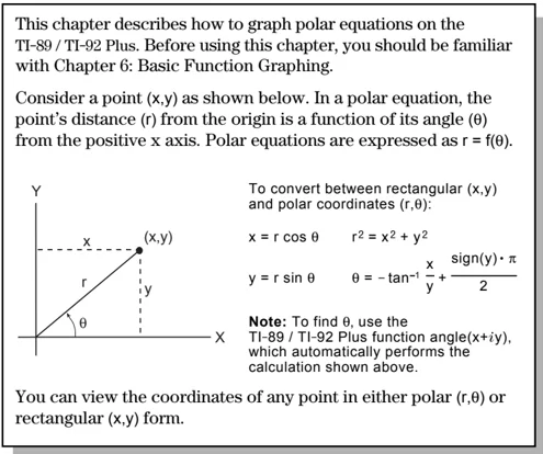
Plots — You can scroll above y1= to see a list of stat plots. See Chapter 16. Function List — You can scroll through the list of functions and definitions. Entry Line — Where you define or edit the function highlighted in the list.
- Press \blacktriangledown and \blacktriangle to move the cursor to any undefined function. (Use [2nd] \blacktriangledown and [2nd] \blacktriangle to scroll one page at a time.)
Tip: For an undefined function, you do not need to press [ENTER] or [F3]. When you begin typing, the cursor moves to the entry line.
-
Press [ENTER] or [F3] to move the cursor to the entry line.
-
Type the expression to define the function.
- The independent variable in function graphing is x.
- The expression can refer to other variables, including matrices, lists, and other functions. Only floats and lists of floats will produce a plot.
-
When you complete the expression, press [ENTER].
The function list now shows the new function, which is automatically selected for graphing.
Editing a Function
From the Y= Editor:
-
Press \blacktriangledown and \blacktriangle to highlight the function.
-
Press [ENTER] or [F3] to move the cursor to the entry line.
-
Do any of the following.
- Use \blacktriangleright and \blacktriangleleft to move the cursor within the expression and edit it. Refer to "Editing an Expression in the Entry Line" in Chapter 2. — or —
- Press [CLEAR] once or twice to clear the old expression, and then type the new one.
-
Press [ENTER].
The function list now shows the edited function, which is automatically selected for graphing.
Tip: If you accidentally move the cursor to the entry line, press [ESC] to move it back to the function list.
Tip: To cancel any editing changes, press [ESC] instead of [ENTER].
Chapter 6: Basic Function Graphing 109
Clearing a Function
From the Y= Editor:
| To erase: | Do this: |
|---|---|
| A function from the function list | Highlight the function and press ← or CLEAR. |
| A function from the entry line | Press CLEAR once or twice (depending on the cursor’s location) and then press ENTER. |
| All functions | Press F1 and then select 8:Clear Functions. When prompted for confirmation, press ENTER. |
Note: F1 8 does not erase any stat plots (Chapter 16).
You don’t have to clear a function to prevent it from being graphed. As described on page 111, you can select the functions you want to graph.
Shortcuts to Move the Cursor
From the Y=Editor:
| Press: | To: |
|---|---|
◆ ← or ◆ → |
Go to function 1 or to the last defined function, respectively. If the cursor is on or past the last defined function, ◆ → goes to function 99. |
From the Home Screen or a Program
You can also define and evaluate a function from the Home screen or a program.
- Use the Define and Graph commands. Refer to:
- “Graphing a Function Defined on the Home Screen” and “Graphing a Piecewise Defined Function” in Chapter 12.
- “Overview of Entering a Function” in Chapter 17.
- Store an expression directly to a function variable. Refer to:
- “Storing and Recalling Variable Values” in Chapter 2.
- “Creating and Evaluating User-Defined Functions” in Chapter 5.
Tip: User-defined functions can have almost any name. However, if you want them to appear in the Y= Editor, use function names y1(x), y2(x), etc.
110 Chapter 6: Basic Function Graphing
Selecting Functions to Graph
Regardless of how many functions are defined in the Y= Editor, you can select the ones you want to graph.
Selecting or Deselecting Functions
Press [Y=] or [APPS] 2 to display the Y= Editor.
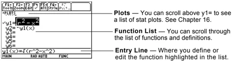
A “✓” indicates which functions will be graphed the next time you display the Graph screen.
If PLOT numbers are displayed, those stat plots are selected.
In this example, Plots 1 and 2 are selected. To view them, scroll above y1=.
Tip: You don't have to select a function when you enter or edit it; it is selected automatically.
Tip: To turn off any stat plots, press [F5] 5 or use [F4] to deselect them.
| To select or deselect: | Do this: |
|---|---|
| A specified function | 1. Move the cursor to highlight the function.2. Press [F4].This procedure selects a deselected function or deselects a selected function. |
| All functions | 1. Press [F5] to display the All toolbar menu.2. Select the applicable item. |
From the Home Screen or a Program
You can also select or deselect functions from the Home screen or a program.
- Use the FnOn and FnOff commands (available from the Home screen’s
[F4]Other toolbar menu) for functions. Refer to Appendix A. - Use the PlotsOn and PlotsOff commands for stat plots. Refer to Appendix A.
Chapter 6: Basic Function Graphing 111
Setting the Display Style for a Function
For each defined function, you can set a style that specifies how that function will be graphed. This is useful when graphing multiple functions. For example, set one as a solid line, another as a dotted line, etc.
Displaying or Changing a Function’s Style
From the Y= Editor:
- Move the cursor to highlight the applicable function.
- Select the Style menu:
- TI-89: Press
[2nd] [F6]. - TI-92 Plus: Press
[F6].
- TI-89: Press

-   Although the Line item is initially highlighted, the function’s current style is indicated by a ✓ mark.
-   To exit the menu without making a change, press `[ESC]`.
- To make a change, select the applicable style.
| Style | Description |
|---|---|
| Line | Connects plotted points with a line. This is the default. |
| Dot | Displays a dot at each plotted point. |
| Square | Displays a solid box at each plotted point. |
| Thick | Connects plotted points with a thick line. |
| Animate | A round cursor moves along the leading edge of the graph but does not leave a path. |
| Path | A round cursor moves along the leading edge of the graph and does leave a path. |
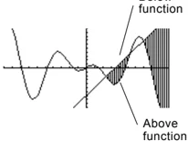
| Above | Shades the area above the graph. |
| Below | Shades the area below the graph. |
Tip: To set Line as the style for all functions, press [F5] and select 4:Reset Styles.
If You Use Above or Below Shading
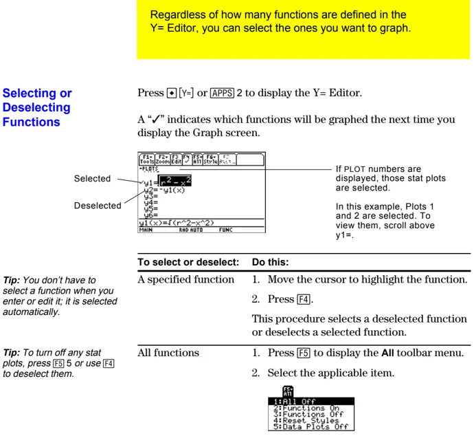
The TI-89 / TI-92 Plus has four shading patterns, used on a rotating basis. If you set one function as shaded, it uses the first pattern. The next shaded function uses the second pattern, etc. The fifth shaded function reuses the first pattern.
When shaded areas intersect, their patterns overlap.
From the Home Screen or a Program
You can also set a function’s style from the Home screen or a program. Refer to the Style command in Appendix A.
112 Chapter 6: Basic Function Graphing
Defining the Viewing Window
The viewing window represents the portion of the coordinate plane displayed on the Graph screen. By setting Window variables, you can define the viewing window’s boundaries and other attributes. Function graphs, parametric graphs, etc., have their own independent set of Window variables.
Displaying Window Variables in the Window Editor
Press □ [WINDOW] or [APPS] 3 to display the Window Editor.
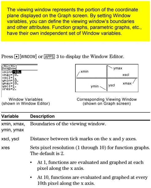
Window Variables
(shown in Window Editor)
Corresponding Viewing Window
(shown on Graph screen)
| Variable | Description |
|---|---|
| xmin, xmax, ymin, ymax | Boundaries of the viewing window. |
| xscl, yscl | Distance between tick marks on the x and y axes. |
| xres | Sets pixel resolution (1 through 10) for function graphs. The default is 2.• At 1, functions are evaluated and graphed at each pixel along the x axis.• At 10, functions are evaluated and graphed at every 10th pixel along the x axis. |
Tip: To turn off tick marks, set xscl=0 and/or yscl=0.
Tip: Small values of xres improve the graph’s resolution but may reduce the graphing speed.
Changing the Values
From the Window Editor:
- Move the cursor to highlight the value you want to change.
- Do any of the following:
- Type a value or an expression. The old value is erased when you begin typing. — or —
- Press [CLEAR] to clear the old value; then type the new one. — or —
- Press ◀ or ▶ to remove the highlighting; then edit the value.
Values are stored as you type them; you do not need to press [ENTER]. [ENTER] simply moves the cursor to the next Window variable.
Note: If you type an expression, it is evaluated when you move the cursor to a different Window variable or leave the Window Editor.
From the Home Screen or a Program
You can also store values directly to the Window variables from the Home screen or a program. Refer to “Storing and Recalling Variable Values” in Chapter 2.
Chapter 6: Basic Function Graphing 113
Changing the Graph Format
You can set the graph format to show or hide reference elements such as the axes, a grid, and the cursor’s coordinates. Function graphs, parametric graphs, etc., have their own independent set of graph formats.
Displaying Graph Format Settings
Tip: You also can display the GRAPH FORMATS dialog box from the Y= Editor, Window Editor, or Graph screen. Press:
TI-89: [♦] [F1]
TI-92 Plus: [♦] F
From the Y= Editor, Window Editor, or Graph screen, press [F1] and select 9:Format.

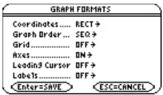
- The GRAPH FORMATS dialog box shows the current settings.
- To exit without making a change, press [ESC].
| Format | Description |
|---|---|
| Coordinates | Shows cursor coordinates in rectangular (RECT) or polar (POLAR) form, or hides (OFF) the coordinates. |
| Graph Order | Graphs functions one at a time (SEQ) or all at the same time (SIMUL). |
| Grid | Shows (ON) or hides (OFF) grid points that correspond to the tick marks on the axes. |
| Axes | Shows (ON) or hides (OFF) the x and y axes. |
| Leading Cursor | Shows (ON) or hides (OFF) a reference cursor that tracks the functions as they are graphed. |
| Labels | Shows (ON) or hides (OFF) labels for the x and y axes. |
Tip: To turn off tick marks, define the viewing window so that xscl and/or yscl = 0.
Changing Settings
From the GRAPH FORMATS dialog box:
- Move the cursor to highlight the format setting.
- Press [♦] to display a menu of valid settings for that format.
- Select a setting. Either:
- Move the cursor to highlight the setting, and then press [ENTER]. — or —
- Press the number for that setting.
- After changing all applicable format settings, press [ENTER] to save your changes and close the GRAPH FORMATS dialog box.
Tip: To cancel a menu or exit the dialog box without saving any changes, use [ESC] instead of [ENTER].
114 Chapter 6: Basic Function Graphing
Graphing the Selected Functions
When you are ready to graph the selected functions, display the Graph screen. This screen uses the display style and viewing window that you previously defined.
Displaying the Graph Screen
Press \blacklozenge [GRAPH] or [APPS] 4. The TI-89 / TI-92 Plus automatically graphs the selected functions.
Note: If you select an [F2] Zoom operation from the Y= Editor or Window Editor, the TI-89 / TI-92 Plus automatically displays the Graph screen.
 BUSY indicator shows while graphing is in progress.
Interrupting Graphing
While graphing is in progress:
- To pause graphing temporarily, press [ENTER]. (The PAUSE indicator replaces BUSY.) To resume, press [ENTER] again.
- To cancel graphing, press [ON]. To start graphing again from the beginning, press [F4] (ReGraph).
If You Need to Change the Viewing Window
Depending on various settings, a function may be graphed such that it is too small, too large, or offset too far to one side of the screen. To correct this:
- Redefine the viewing window with different boundaries (page 113).
- Use a Zoom operation (page 119).
Smart Graph
When you display the Graph screen, the Smart Graph feature displays the previous window contents immediately, provided nothing has changed that requires regraphing.
Smart Graph updates the window and regraphs only if you have:
- Changed a mode setting that affects graphing, a function's graphing attribute, a Window variable, or a graph format.
- Selected or deselected a function or stat plot. (If you only select a new function, Smart Graph adds that function to the Graph screen.)
- Changed the definition of a selected function or the value of a variable in a selected function.
- Cleared a drawn object (Chapter 12).
- Changed a stat plot definition (Chapter 16).
Chapter 6: Basic Function Graphing 115
Displaying Coordinates with the Free-Moving Cursor
To display the coordinates of any location on the Graph screen, use the free-moving cursor. You can move the cursor to any pixel on the screen; the cursor is not confined to a graphed function.
Free-Moving Cursor
When you first display the Graph screen, no cursor is visible. To display the cursor, press a cursor pad arrow. The cursor moves from the center of the screen, and its coordinates are displayed.
Tip: If your screen does not show coordinates, set the graph format so that Coordinates = RECT or POLAR. Press: TI-89: [♦] [1] TI-92 Plus: [♦] F
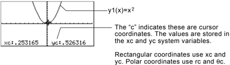
The “c” indicates these are cursor coordinates. The values are stored in the xc and yc system variables.
Rectangular coordinates use xc and yc. Polar coordinates use rc and θc.
Tip: To hide the cursor and its coordinates temporarily, press [CLEAR], [ESC], or [ENTER]. The next time you move the cursor, it moves from its last position.
| To move the free-moving cursor: | Press: |
|---|---|
| To an adjoining pixel | A cursor pad arrow for any direction. |
| In increments of 10 pixels | [2nd] and then a cursor pad arrow. |
When you move the cursor to a pixel that appears to be “on” the function, it may be near the function but not on it.
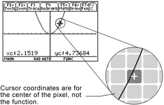
Cursor coordinates are for the center of the pixel, not the function.
To increase the accuracy:
- Use the Trace tool described on the next page to display coordinates that are on the function.
- Use a Zoom operation to zoom in on a portion of the graph.
116 Chapter 6: Basic Function Graphing
Tracing a Function
To display the exact coordinates of any plotted point on a graphed function, use the [F3] Trace tool. Unlike the free-moving cursor, the trace cursor moves only along a function’s plotted points.
Beginning a Trace
From the Graph screen, press [F3].
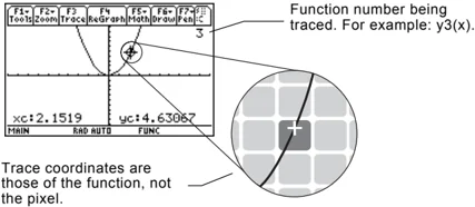
The trace cursor appears on the function, at the middle x value on the screen. The cursor’s coordinates are displayed at the bottom of the screen.
If multiple functions are graphed, the trace cursor appears on the lowest-numbered function selected in the Y= Editor. The function number is shown in the upper right part of the screen.
Note: If any stat plots are graphed (Chapter 16), the trace cursor appears on the lowest-numbered stat plot.
Moving along a Function
| To move the trace cursor: | Do this: |
|---|---|
| To the previous or next plotted point | Press ◀ or ▶. |
| Approximately 5 plotted points (it may be more or less than 5, depending on the xres Window variable) | Press [2nd] ◀ or [2nd] ▶. |
| To a specified x value on the function | Type the x value and press [ENTER]. |
The trace cursor moves only from plotted point to plotted point along the function, not from pixel to pixel.
Note: If you enter an x value, it must be between xmin and xmax.
Tip: If your screen does not show coordinates, set the graph format so that Coordinates = RECT or POLAR. Press: TI-89: [♦] [F] TI-92 Plus: [♦] F

Trace coordinates are those of the function, not the pixel.
Each displayed y value is calculated from the x value; that is, y=yn(x). If the function is undefined at an x value, the y value is blank.
You can continue to trace a function that goes above or below the viewing window. You cannot see the cursor as it moves in that “off the screen” area, but the displayed coordinate values show its correct coordinates.
Tip: Use QuickCenter, described on the next page, to trace a function that goes above or below the window.
Chapter 6: Basic Function Graphing 117
Moving from Function to Function
Press \odot or \odot to move to the previous or next selected function at the same x value. The new function number is shown on the screen.
The “previous or next” function is based on the order of the selected functions in the Y= Editor, not the appearance of the functions as graphed on the screen.
Automatic Panning
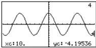
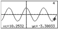
If you trace a function off the left or right edge of the screen, the viewing window automatically pans to the left or right. There is a slight pause while the new portion of the graph is drawn.
Note: Automatic panning does not work if stat plots are displayed or if a function uses a shaded display style.
Before automatic pan After automatic pan
After an automatic pan, the cursor continues tracing.
Using QuickCenter
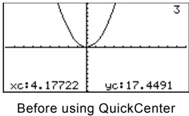
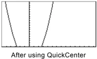
If you trace a function off the top or bottom of the viewing window, you can press ENTER to center the viewing window on the cursor location.
Tip: You can use QuickCenter at any time during a trace, even when the cursor is still on the screen.
Before using QuickCenter After using QuickCenter
After QuickCenter, the cursor stops tracing. If you want to continue tracing, press F3.
Canceling Trace
To cancel a trace at any time, press ESC.
A trace is also canceled when you display another application screen such as the Y= Editor. When you return to the Graph screen and press F3 to begin tracing:
- If Smart Graph regraphed the screen, the cursor appears at the middle x value.
- If Smart Graph does not regraph the screen, the cursor appears at its previous location (before you displayed the other application).
118 Chapter 6: Basic Function Graphing
Using Zooms to Explore a Graph
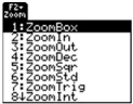
The F2 Zoom toolbar menu has several tools that let you adjust the viewing window. You can also save a viewing window for later use.
Overview of the Zoom Menu
Press F2 from the Y= Editor, Window Editor, or Graph screen.
Note: If you select a Zoom tool from the Y=Editor or Window Editor, the TI-89 / TI-92 Plus automatically displays the Graph screen.
Procedures for using ZoomBox, ZoomIn, ZoomOut, ZoomStd, Memory, and SetFactors are given later in this section.
For more information about the other items, refer to Appendix A.
Note: x and y are the distances from the center of one pixel to the center of an adjoining pixel.
Chapter 6: Basic Function Graphing 119
Zooming In with a Zoom Box
Tip: To move the cursor in larger increments, use 2nd 0, 2nd , etc.
-
From the F2 Zoom menu, select 1:ZoomBox. The screen prompts for 1st Corner?
-
Move the cursor to any corner of the box you want to define, and then press ENTER. The cursor changes to a small square, and the screen prompts for 2nd Corner?
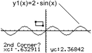
- Move the cursor to the opposite corner of the zoom box. As you move the cursor, the box stretches.
Tip: You can cancel ZoomBox by pressing ESC before you press ENTER.
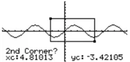
- When you have outlined the area you want to zoom in on, press ENTER. The Graph screen shows the zoomed area.
Zooming In and Out on a Point
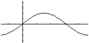
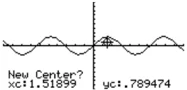
- From the F2 Zoom menu, select 2:ZoomIn or 3:ZoomOut. A cursor appears, and the screen prompts for New Center?
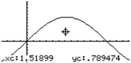
- Move the cursor to the point where you want to zoom in or out, and then press ENTER. The TI-89 / TI-92 Plus adjusts the Window variables by the Zoom factors defined in SetFactors.
- For a ZoomIn, the x variables are divided by xFact, and the y variables are divided by yFact. new xmin = xmin / xFact , etc.
- For a ZoomOut, the x variables are multiplied by xFact, and the y variables are multiplied by yFact. new xmin = xmin * xFact , etc.
120 Chapter 6: Basic Function Graphing
Changing Zoom Factors
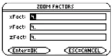
The Zoom factors define the magnification and reduction used by ZoomIn and ZoomOut.
- From the \boxedF2 Zoom menu, select C:SetFactors to display the ZOOM FACTORS dialog box.
Tip: To exit without saving any changes, press \boxedESC.
Zoom factors must be ≥ 1, but they do not have to be integers. The default setting is 4.
-
Use \ominus and \oplus to highlight the value you want to change. Then:
- Type the new value. The old value is cleared automatically when you begin typing. — or —
- Press \textcircled\leftarrow or \textcircled\rightarrow to remove the highlighting, and then edit the old value.
-
Press \boxedENTER (after typing in an input box, you must press \boxedENTER twice) to save any changes and exit the dialog box.
Saving or Recalling a Viewing Window
After using various Zoom tools, you may want to return to a previous viewing window or save the current one.
- From the \boxedF2 Zoom menu, select B:Memory to display its submenu.

- Select the applicable item.
Note: You can store only one set of Window variable values at a time. Storing a new set overwrites the old set.
Restoring the Standard Viewing Window
You can restore the Window variables to their default values at any time.
From the \boxedF2 Zoom menu, select 6:ZoomStd.
Chapter 6: Basic Function Graphing 121
Using Math Tools to Analyze Functions
On the Graph screen, the [F5] Math toolbar menu has several tools that help you analyze graphed functions.
Overview of the Math Menu
Press [F5] from the Graph screen.
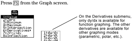
Note: For Math results, cursor coordinates are stored in system variables xc and yc (rc and θc if you use polar coordinates). Derivatives, integrals, distances, etc., are stored in the system variable sysMath.
| Math Tool | Description |
|---|---|
| Value | Evaluates a selected y(x) function at a specified x value. |
| Zero, Minimum, Maximum | Finds a zero (x-intercept), minimum, or maximum point within an interval. |
| Intersection | Finds the intersection of two functions. |
| Derivatives | Finds the derivative (slope) at a point. |
| ∫f(x)dx | Finds the approximate numerical integral over an interval. |
| Inflection | Finds the inflection point of a curve, where its second derivative changes sign (where the curve changes concavity). |
| Distance | Draws and measures a line between two points on the same function or on two different functions. |
| Tangent | Draws a tangent line at a point and displays its equation. |
| Arc | Finds the arc length between two points along a curve. |
| Shade | Depends on the number of functions graphed.• If only one function is graphed, this shades the function’s area above or below the x axis.• If two or more functions are graphed, this shades the area between any two functions within an interval. |
122 Chapter 6: Basic Function Graphing
Finding y(x) at a Specified Point
- From the Graph screen, press F5 and select 1:Value.
- Type the x value, which must be a real value between xmin and xmax. The value can be an expression.
- Press ENTER.
The cursor moves to that x value on the first function selected in the Y= Editor, and its coordinates are displayed.
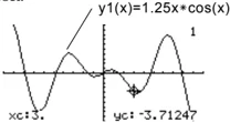
- Press \ominus or \oplus to move the cursor between functions at the entered x value. The corresponding y value is displayed.
Note: If you press \blacktriangleleft or \blacktriangleright, the free-moving cursor appears. You may not be able to move it back to the entered x value.
Tip: You can also display function coordinates by tracing the function (F3), typing an x value, and pressing ENTER.
Finding a Zero, Minimum, or Maximum within an Interval
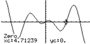
- From the Graph screen, press F5 and select 2:Zero, 3:Minimum, or 4:Maximum.
- As necessary, use \ominus and \oplus to select the applicable function.
- Set the lower bound for x. Either use \blacktriangleleft and \blacktriangleright to move the cursor to the lower bound or type its x value.
- Press ENTER. A \blacktriangleright at the top of the screen marks the lower bound.
- Set the upper bound, and press ENTER.
The cursor moves to the solution, and its coordinates are displayed.
Tip: Typing x values is a quick way to set bounds.
Finding the Intersection of Two Functions within an Interval
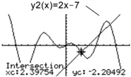
- From the Graph screen, press F5 and select 5:Intersection.
- Select the first function, using \ominus or \oplus as necessary, and press ENTER. The cursor moves to the next graphed function.
- Select the second function, and press ENTER.
- Set the lower bound for x. Either use \blacktriangleleft and \blacktriangleright to move the cursor to the lower bound or type its x value.
- Press ENTER. A \blacktriangleright at the top of the screen marks the lower bound.
- Set the upper bound, and press ENTER.
The cursor moves to the intersection, and its coordinates are displayed.
Chapter 6: Basic Function Graphing 123
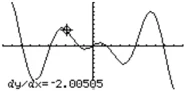
Finding the Derivative (Slope) at a Point
- From the Graph screen, press F5 and select 6:Derivatives. Then select 1:dy/dx from the submenu.
- As necessary, use \ominus and \oplus to select the applicable function.
- Set the derivative point. Either move the cursor to the point or type its x value.
- Press ENTER.
The derivative at that point is displayed.
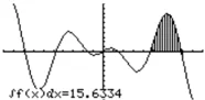
Finding the Numerical Integral over an Interval
Tip: Typing x values is a quick way to set the limits.
- From the Graph screen, press F5 and select 7:∫f(x)dx.
- As necessary, use \ominus and \oplus to select the applicable function.
- Set the lower limit for x. Either use ◂ and ▸ to move the cursor to the lower limit or type its x value.
- Press ENTER. A ▸ at the top of the screen marks the lower limit.
- Set the upper limit, and press ENTER.
The interval is shaded, and its approximate numerical integral is displayed.
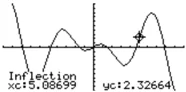
Tip: To erase the shaded area, press F4 (ReGraph).
Finding an Inflection Point within an Interval
- From the Graph screen, press F5 and select 8:Inflection.
- As necessary, use \ominus and \oplus to select the applicable function.
- Set the lower bound for x. Either use ◂ and ▸ to move the cursor to the lower bound or type its x value.
- Press ENTER. A ▸ at the top of the screen marks the lower bound.
- Set the upper bound, and press ENTER.
The cursor moves to the inflection point (if any) within the interval, and its coordinates are displayed.
124 Chapter 6: Basic Function Graphing
Finding the Distance between Two Points
- From the Graph screen, press F5 and select 9:Distance.
- As necessary, use \odot and \ominus to select the function for the first point.
- Set the first point. Either use \textcircled4 or \textcircled5 to move the cursor to the point or type its x value.
- Press ENTER. A + marks the point.
- If the second point is on a different function, use \odot and \ominus to select the function.
- Set the second point. (If you use the cursor to set the point, a line is drawn as you move the cursor.)
- Press ENTER.
The distance between the two points is displayed, along with the connecting line.
 Distance=10.5937
Drawing a Tangent Line
Tip: To erase a drawn tangent line, press F4 (ReGraph).
- From the Graph screen, press F5 and select A:Tangent.
- As necessary, use \odot and \ominus to select the applicable function.
- Set the tangent point. Either move the cursor to the point or type its x value.
- Press ENTER.
The tangent line is drawn, and its equation is displayed.
 y=-2.93453x+4.83823
Finding an Arc Length
- From the Graph screen, press F5 and select B:Arc.
- As necessary, use \odot and \ominus to select the applicable function.
- Set the first point of the arc. Either use \textcircled4 or \textcircled5 to move the cursor or type the x value.
- Press ENTER. A + marks the first point.
- Set the second point, and press ENTER.
A + marks the second point, and the arc length is displayed.
 Arc=12.6638
Chapter 6: Basic Function Graphing 125
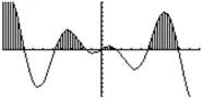
Shading the Area between a Function and the X Axis
You must have only one function graphed. If you graph two or more functions, the Shade tool shades the area between two functions.
- From the Graph screen, press F5 and select C:Shade. The screen prompts for Above X axis?
- Select one of the following. To shade the function's area:
- Above the x axis, press ENTER.
- Below the x axis, press: TI-89: alpha [N] TI-92 Plus: N
- Set the lower bound for x. Either use 4 and 9 to move the cursor to the lower bound or type its x value.
- Press ENTER. A ▶ at the top of the screen marks the lower bound.
- Set the upper bound, and press ENTER.
The bounded area is shaded.
Note: If you do not press 4 or 9, or type an x value when setting the lower and upper bound, xmin and xmax will be used as the lower and upper bound, respectively.
Tip: To erase the shaded area, press F4 (ReGraph).
Shading the Area between Two Functions within an Interval
You must have at least two functions graphed. If you graph only one function, the Shade tool shades the area between the function and the x axis.
- From the Graph screen, press F5 and select C:Shade. The screen prompts for Above?
- As necessary, use ⌖ or ⊕ to select a function. (Shading will be above this function.)
- Press ENTER. The cursor moves to the next graphed function, and the screen prompts for Below?
- As necessary, use ⌖ or ⊕ to select another function. (Shading will be below this function.)
- Press ENTER.
- Set the lower bound for x. Either use 4 and 9 to move the cursor to the lower bound or type its x value.
- Press ENTER. A ▶ at the top of the screen marks the lower bound.
- Set the upper bound, and press ENTER.
The bounded area is shaded.
Note: If you do not press 4 or 9, or type an x value when setting the lower and upper bound, xmin and xmax will be used as the lower and upper bound, respectively.
Tip: To erase the shaded area, press F4 (ReGraph).
126 Chapter 6: Basic Function Graphing
Parametric Graphing
7
- Preview of Parametric Graphing ........ 128
- Overview of Steps in Graphing Parametric Equations ........ 129
- Differences in Parametric and Function Graphing ........ 130
This chapter describes how to graph parametric equations on the TI-89 / TI-92 Plus. Before using this chapter, you should be familiar with Chapter 6: Basic Function Graphing.
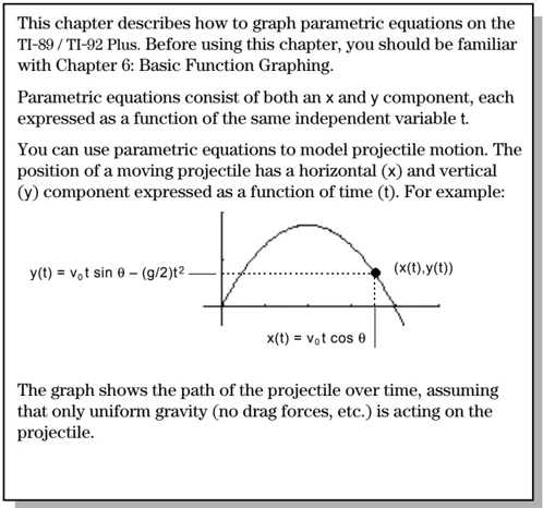
Parametric equations consist of both an x and y component, each expressed as a function of the same independent variable t.
You can use parametric equations to model projectile motion. The position of a moving projectile has a horizontal (x) and vertical (y) component expressed as a function of time (t). For example:

The graph shows the path of the projectile over time, assuming that only uniform gravity (no drag forces, etc.) is acting on the projectile.
Chapter 7: Parametric Graphing 127
Preview of Parametric Graphing
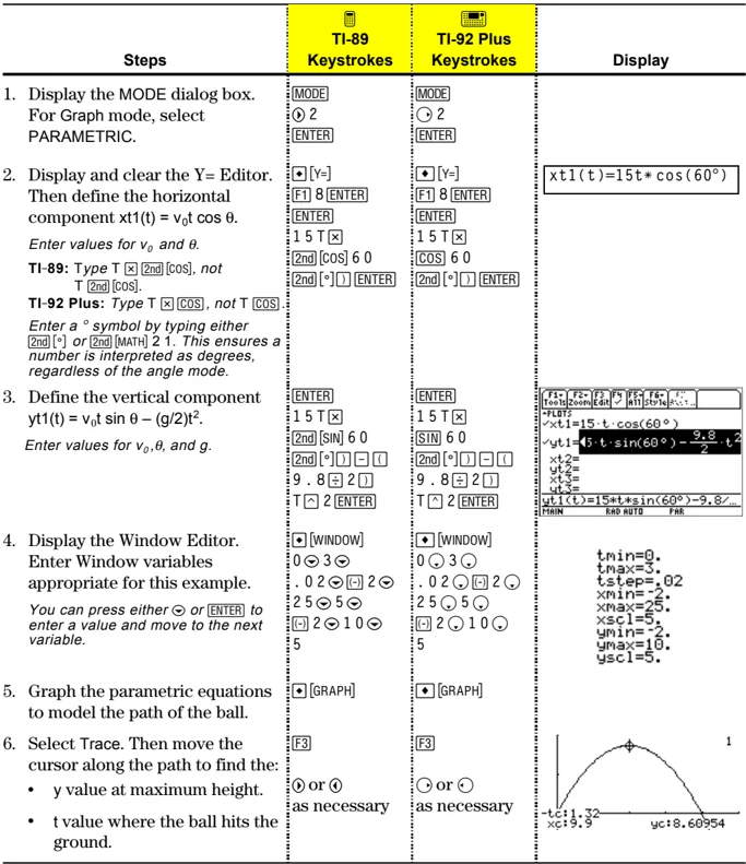
Graph the parametric equations describing the path of a ball kicked at an angle (θ) of 60° with an initial velocity (v₀) of 15 meters/sec. The gravity constant g = 9.8 meters/sec². Ignoring air resistance and other drag forces, what is the maximum height of the ball and when does it hit the ground?
| Steps | TI-89 Keystrokes | TI-92 Plus Keystrokes | Display |
|---|---|---|---|
| 1. Display the MODE dialog box. For Graph mode, select PARAMETRIC. | [MODE] ◯ 2 [ENTER] | [MODE] ◯ 2 [ENTER] | |
| 2. Display and clear the Y= Editor. Then define the horizontal component xt1(t) = v₀t cos θ. Enter values for v₀ and θ. TI-89: Type T × [2nd] [COS], not T [2nd] [COS]. TI-92 Plus: Type T × [COS], not T [COS]. Enter a ° symbol by typing either [2nd] [°] or [2nd] [MATH] 2 1. This ensures a number is interpreted as degrees, regardless of the angle mode. | ◆ [Y=] [F1] 8 [ENTER] [ENTER] 1 5 T × [2nd] [COS] 6 0 [2nd] [°] [ ) ] [ENTER] | ◆ [Y=] [F1] 8 [ENTER] [ENTER] 1 5 T × [COS] 6 0 [2nd] [°] [ ) ] [ENTER] | xt1(t)=15t*cos(60°) |
| 3. Define the vertical component yt1(t) = v₀t sin θ – (g/2)t². Enter values for v₀, θ, and g. | [ENTER] 1 5 T × [2nd] [SIN] 6 0 [2nd] [°] [ ) ] – [ ( ] 9 . 8 ÷ 2 [ ) ] T ^ 2 [ENTER] | [ENTER] 1 5 T × [SIN] 6 0 [2nd] [°] [ ) ] – [ ( ] 9 . 8 ÷ 2 [ ) ] T ^ 2 [ENTER] | |
| 4. Display the Window Editor. Enter Window variables appropriate for this example. You can press either ◯ or [ENTER] to enter a value and move to the next variable. | ◆ [WINDOW] 0 ◯ 3 ◯ . 0 2 ◯ [(-)] 2 ◯ 2 5 ◯ 5 ◯ [(-)] 2 ◯ 1 0 ◯ 5 | ◆ [WINDOW] 0 ◯ 3 ◯ . 0 2 ◯ [(-)] 2 ◯ 2 5 ◯ 5 ◯ [(-)] 2 ◯ 1 0 ◯ 5 | tmin=0. tmax=3. tstep=.02 xmin=-2. xmax=25. xscl=5. ymin=-2. ymax=10. yscl=5. |
| 5. Graph the parametric equations to model the path of the ball. | ◆ [GRAPH] | ◆ [GRAPH] | |
| 6. Select Trace. Then move the cursor along the path to find the: • y value at maximum height. • t value where the ball hits the ground. | [F3] ◯ or ◯ as necessary | [F3] ◯ or ◯ as necessary |
128 Chapter 7: Parametric Graphing
Overview of Steps in Graphing Parametric Equations
To graph parametric equations, use the same general steps used for y(x) functions as described in Chapter 6: Basic Function Graphing. Any differences that apply to parametric equations are described on the following pages.
Graphing Parametric Equations
Set Graph mode ([MODE]) to PARAMETRIC. Also set Angle mode, if necessary.
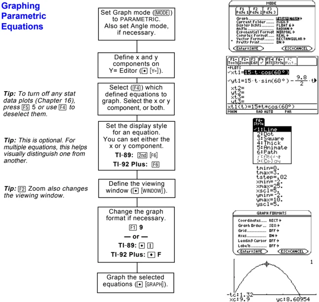
Tip: To turn off any stat data plots (Chapter 16), press [F5] 5 or use [F4] to deselect them.
Select ([F4]) which defined equations to graph. Select the x or y component, or both.
Tip: This is optional. For multiple equations, this helps visually distinguish one from another.
Set the display style for an equation. You can set either the x or y component. TI-89: [2nd] [F6] TI-92 Plus: [F6]
Tip: [F2] Zoom also changes the viewing window.
Define the viewing window ([♦] [WINDOW]).
Change the graph format if necessary. [F1] 9 — or — TI-89: [♦] [1] TI-92 Plus: [♦] F
Graph the selected equations ([♦] [GRAPH]).
Exploring the Graph
From the Graph screen, you can:
- Display the coordinates of any pixel by using the free-moving cursor, or of a plotted point by tracing a parametric equation.
- Use the [F2] Zoom toolbar menu to zoom in or out on a portion of the graph.
- Use the [F5] Math toolbar menu to find derivatives, tangents, etc. Some menu items are not available for parametric graphs.
Chapter 7: Parametric Graphing 129
Differences in Parametric and Function Graphing
This chapter assumes that you already know how to graph y(x) functions as described in Chapter 6: Basic Function Graphing. This section describes the differences that apply to parametric equations.
Setting the Graph Mode
Use [MODE] to set Graph = PARAMETRIC before you define equations or set Window variables. The Y= Editor and the Window Editor let you enter information for the current Graph mode setting only.
Defining Parametric Equations on the Y= Editor
To graph a parametric equation, you must define both its x and y components. If you define only one component, the equation cannot be graphed. (However, you can use single components to generate an automatic table as described in Chapter 13.)
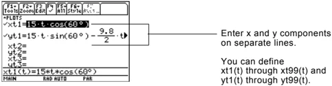
Enter x and y components on separate lines.
You can define xt1(t) through xt99(t) and yt1(t) through yt99(t).
Be careful when using implied multiplication with t. For example:
| Enter: | Instead of: | Because: |
|---|---|---|
| t*cos(60) | tcos(60) | tcos is interpreted as a user-defined function called tcos, not as implied multiplication. |
| In most cases, this refers to a nonexistent function. So the TI-89 / TI-92 Plus simply returns the function name, not a number. |
Note: When using t, be sure implied multiplication is valid for your situation.
Tip: You can use the Define command from the Home screen (see Appendix A) to define functions and equations for any graphing mode, regardless of the current mode.
The Y= Editor maintains an independent function list for each Graph mode setting. For example, suppose:
- In FUNCTION graphing mode, you define a set of y(x) functions. You change to PARAMETRIC graphing mode and define a set of x and y components.
- When you return to FUNCTION graphing mode, your y(x) functions are still defined in the Y= Editor. When you return to PARAMETRIC graphing mode, your x and y components are still defined.
130 Chapter 7: Parametric Graphing
To graph a parametric equation, select either its x or y component or both. When you enter or edit a component, it is selected automatically.
Selecting Parametric Equations
Selecting x and y components separately can be useful for tables as described in Chapter 13. With multiple parametric equations, you can select and compare all the x components or all the y components.
Selecting the Display Style
You can set the style for either the x or y component. For example, if you set the x component to Dot, the TI-89 / TI-92 Plus automatically sets the y component to Dot.
Tip: Use the Animate and Path styles for interesting projectile-motion effects.
The Above and Below styles are not available for parametric equations and are dimmed on the Y= Editor's Style toolbar menu.
Window Variables
The Window Editor maintains an independent set of Window variables for each Graph mode setting (just as the Y= Editor maintains independent function lists). Parametric graphs use the following Window variables.
\begin{tabular}{ll} Variable & Description \ tmin, tmax & Smallest and largest t values to evaluate. \ tstep & Increment for the t value. Parametric equations are evaluated at: \ & \quad x(tmin) \quad \quad \quad \quad \quad y(tmin) \ & \quad x(tmin+tstep) \quad \quad y(tmin+tstep) \ & \quad x(tmin+2(tstep)) \quad y(tmin+2(tstep)) \ & \quad ... not to exceed ... \quad ... not to exceed ... \ & \quad x(tmax) \quad \quad \quad \quad \quad y(tmax) \ xmin, xmax, ymin, ymax & Boundaries of the viewing window. \ xscl, yscl & Distance between tick marks on the x and y axes. \ \end{tabular}
Note: You can use a negative tstep. If so, tmin must be greater than tmax.
Standard values (set when you select 6:ZoomStd from the F2 Zoom toolbar menu) are:
tmin = 0. \quad \quad \quad \quad \quad \quad \quad \quad \quad \quad \quad \quad xmin = -10. \quad \quad ymin = -10. tmax = 2\pi (6.2831853... radians \quad \quad xmax = 10. \quad \quad ymax = 10. \quad \quad \quad \quad \quad \quad \quad \quad \quad \quad \quad or 360 degrees) tstep =\pi/24 (.1308996... radians \quad \quad xscl = 1. \quad \quad yscl = 1. \quad \quad \quad \quad \quad \quad \quad \quad \quad \quad \quad or 7.5 degrees)
You may need to change the standard values for the t variables (tmin, tmax, tstep) to ensure that enough points are plotted.
Chapter 7: Parametric Graphing 131
Exploring a Graph
As in function graphing, you can explore a graph by using the following tools.
Tip: During a trace, you can also evaluate x(t) and y(t) by typing the t value and pressing ENTER.
Tip: You can use QuickCenter at any time during a trace, even if the cursor is still on the screen.
132 Chapter 7: Parametric Graphing
Polar Graphing
8
- Preview of Polar Graphing ........ 134
- Overview of Steps in Graphing Polar Equations ........ 135
- Differences in Polar and Function Graphing ........ 136
This chapter describes how to graph polar equations on the TI-89 / TI-92 Plus. Before using this chapter, you should be familiar with Chapter 6: Basic Function Graphing.
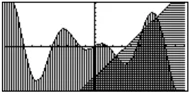
Consider a point (x,y) as shown below. In a polar equation, the point's distance (r) from the origin is a function of its angle (\theta) from the positive x axis. Polar equations are expressed as r = f(\theta).

To convert between rectangular (x,y) and polar coordinates (r,\theta):
x = r \cos \theta $r^2 = x^2 + y^2$
y = r \sin \theta \theta = -\tan^-1 x/y + \fracsign(y) \cdot \pi2
Note: To find \theta, use the TI-89 / TI-92 Plus function angle(x+iy), which automatically performs the calculation shown above.
You can view the coordinates of any point in either polar (r,\theta) or rectangular (x,y) form.
Chapter 8: Polar Graphing 133