Studying the Flight of a Hit Baseball
This activity uses the split screen settings to show a parametric graph and a table at the same time to study the flight of a hit baseball.
Setting Up a Parametric Graph and Table
Perform the following steps to study the flight of a hit baseball that has an initial velocity of 95 feet per second and an initial angle of 32 degrees.
- Set the modes for Page 1 as shown in this screen.
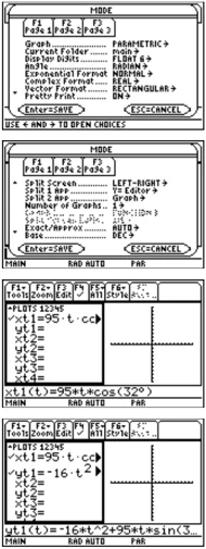
- Set the modes for Page 2 as shown in this screen.
Hint: Press [2nd] [°] to obtain the degree symbol.
-
In the Y= Editor on the left side, enter the equation for the distance of the ball at time t for xt1(t). xt1(t)=95tcos(32°)
-
In the Y= Editor, enter the equation for the height of the ball at time t for yt1(t). yt1(t)=-16t^2+95t*sin(32°)
400 Chapter 23: Activities
- Set the Window variables to: t values= [0,4,.1] x values= [0,300,50] y values= [0,100,10]
Hint: Press \boxed2nd \boxedWINDOW.
- Switch to the right side and display the graph.
Hint: Press \boxedDIAMOND \boxedTblSet.
- Display the TABLE SETUP dialog box, and change tblStart to 0 and \Deltatbl to 0.1.
Hint: Press \boxedDIAMOND \boxedTABLE.
- Display the table in the left side and press \odot to highlight t=2.
Note: As you move the trace cursor from tc=0.0 to tc=3.1, you will see the position of the ball at time tc.
- Switch to the right side. Press \boxedF3, and trace the graph to show the values of xc and yc when tc=2.
Optional Exercise Assuming the same initial velocity of 95 feet per second, find the angle that the ball should be hit to achieve the greatest distance.
Chapter 23: Activities 401

Visualizing Complex Zeros of a Cubic Polynomial
This activity describes graphing the complex zeros of a cubic polynomial. Detailed information about the steps used in this example can be found in Chapter 3: Symbolic Manipulation and Chapter 10: 3D Graphing.
Visualizing Complex Roots
Perform the following steps to expand the cubic polynomial (x-1)(x-i)(x+i), find the absolute value of the function, graph the modulus surface, and use the Trace tool to explore the modulus surface.
-
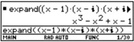
On the Home screen, use the expand() function to expand the cubic expression (x-1)(x-i) (x+i) and see the first polynomial.
-
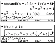
Copy and paste the last answer to the entry line and store it in the function f(x).
-
Use the abs() function to find the absolute value of f(x+yi). (This calculation may take about 2 minutes.)
-
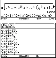
Copy and paste the last answer to the entry line and store it in the function z1(x,y).
-
Set the unit to 3D graph mode, turn on the axes for graph format, and set the Window variables to:
eye= [20,70,0] x= [-2,2,20] y= [-2,2,20] z= [-1,2] ncontour= [5]
Hint: Move the cursor into the history area to highlight the last answer and press ENTER, to copy it to the entry line.
Note: The absolute value of a function forces any roots to visually just touch rather than cross the x axis. Likewise, the absolute value of a function of two variables will force any roots to visually just touch the xy plane.
Note: The graph of z1(x,y) will be the modulus surface.
402 Chapter 23: Activities
Note: Calculating and drawing the graph takes about three minutes.
-
In the Y=Editor, press: TI-89: \boxed◆ \boxedF1 TI-92 Plus: \boxed◆ F and set the Graph Format variables to: Axes= ON Labels= ON Style= HIDDEN SURFACE
-
Graph the modulus surface. The 3D graph is used to visually display a picture of the roots where the surface touches the xy plane.
-
Use the Trace tool to explore the function values at x=1 and y=0.
-
Use the Trace tool to explore the function values at x=0 and y=1.
-
Use the Trace tool to explore the function values at x=0 and y= - 1.
Summary
Note that zc is zero for each of the function values in steps 7–9. Thus, the complex zeros 1, $-i$, $i$ of the polynomial $x^3 - x^2 +x - 1$ can be visualized with the three points where the graph of the modulus surface touches the xy plane.
Chapter 23: Activities 403

Solving a Standard Annuity Problem
This activity can be used to find the interest rate, starting principal, number of compounding periods, and future value of an annuity.
Finding the Interest Rate of an Annuity
Perform the following steps to find the interest rate (i) of an annuity where the starting principal (p) is 1,000, number of compounding periods (n) is 6, and the future value (s) is 2,000.
-
On the Home screen, enter the equation to solve for p.
-
Enter the equation to solve for n.
Tip: To enter the "with" (|) operator: TI-89: [F4] TI-92 Plus: [2nd] [.]
- Enter the equation to solve for i using the "with" operator.
solve(s=p*(1+i)^n,i) | s=2000 and p=1000 and n=6
Result: The interest rate is 12.246%.
Tip: Press [▼] [ENTER] to obtain a floating-point result.
Finding the Future Value of an Annuity
Find the future value of an annuity using the values from the previous example where the interest rate is 14%.
Enter the equation to solve for s.
solve(s=p*(1+i)^n,s)| i=.14 and p=1000 and n=6
Result: The future value at 14% interest is 2,194.97.
404 Chapter 23: Activities


Computing the Time-Value-of-Money
This activity creates a function that can be used to find the cost of financing an item. Detailed information about the steps used in this example can be found in Chapter 17: Programming.
Time-Value-of-Money Function
Tip: You can use your computer keyboard to type lengthy text and then use TI-GRAPH LINK to send it to the TI-89 / TI-92 Plus.
In the Program Editor, define the following Time-Value-of-Money (tvm) function where temp1 = number of payments, temp2 = annual interest rate, temp3 = present value, temp4 = monthly payment, temp5 = future value, and temp6 = begin- or end-of-payment period (1 = beginning of month, 0 = end of month).
:tvm(temp1,temp2,temp3,temp4,temp5,temp6) :Func :Local tempi,tempfunc,tempstr1 :- temp3+(1+temp2/1200* temp6)* temp4* ((1 - (1+temp2/1200)^ ( - temp1))/(temp2/1200))- temp5* (1+temp2/1200)^( - temp1) → tempfunc :For tempi,1,5,1 :"temp"&exact(string(tempi))→ tempstr1 :If when(#tempstr1=0,false,false,true) Then :If tempi=2 :Return approx(nsolve(tempfunc=0,#tempstr1) | #tempstr1>0 and #tempstr1<100) :Return approx(nsolve(tempfunc=0,#tempstr1)) :EndIf :EndFor :Return "parameter error" :EndFunc
Finding the Monthly Payment
Find the monthly payment on 10,000 if you make 48 payments at 10% interest per year.
On the Home screen, enter the tvm values to find pmt.
■ tvm(48,10,10000,pmt,0,1) 251.53 tvm(48,10,10000,pmt,0,1) MAIN RAD AUTO FUNC □/□□
Result: The monthly payment is 251.53.
Finding the Number of Payments
Find the number of payments it will take to pay off the loan if you could make a 300 payment each month.
On the Home screen, enter the tvm values to find n.
■ tvm(n,10,10000,300,0,1) 38.8308 tvm(n,10,10000,300,0,1) MAIN RAD AUTO FUNC □/□□
Result: The number of payments is 38.8308.
Chapter 23: Activities 405


Finding Rational, Real, and Complex Factors
This activity shows how to find rational, real, or complex factors of expressions. Detailed information about the steps used in this example can be found in Chapter 3: Symbolic Manipulation.
Finding Factors
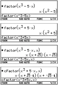
Enter the expressions shown below on the Home screen.
-
factor(x^3 – 5x) [ENTER] displays a rational result.
-
factor(x^3+5x) [ENTER] displays a rational result.
-
factor(x^3 – 5x,x) [ENTER] displays a real result.
-
cfactor(x^3+5x,x) [ENTER] displays a complex result.
406 Chapter 23: Activities
Simulation of Sampling without Replacement
This activity simulates drawing different colored balls from an urn without replacing them. Detailed information about the steps used in this example can be found in Chapter 17: Programming.
Sampling-without-Replacement Function
In the Program Editor, define drawball() as a function that can be called with two parameters. The first parameter is a list where each element is the number of balls of a certain color. The second parameter is the number of balls to select. This function returns a list where each element is the number of balls of each color that were selected.
:drawball(urnlist,drawnum) :Func :Local templist,drawlist,colordim, numballs,i,pick,urncum,j :If drawnum>sum(urnlist) :Return "too few balls" :dim(urnlist)►colordim :urnlist►templist :newlist(colordim)►drawlist :For i,1,drawnum,1 :sum(templist)►numballs :rand(numballs)►pick :For j,1,colordim,1 :cumSum(templist)►urncum (continued in next column)
:If pick ≤ urncum[j] Then :drawlist[j]+1►drawlist[j] :templist[j]- 1►templist[j] :Exit :EndIf :EndFor :EndFor :Return drawlist :EndFunc
Sampling without Replacement
Suppose an urn contains n1 balls of a color, n2 balls of a second color, n3 balls of a third color, etc. Simulate drawing balls without replacing them.
-
Enter a random seed using the RandSeed command.
-
Assuming the urn contains 10 red balls and 25 white balls, simulate picking 5 balls at random from the urn without replacement. Enter drawball({10,25},5).
Result: 2 red balls and 3 white balls.
Chapter 23: Activities 407

408 Chapter 23: Activities
Functions and Instructions
A
- Quick-Find Locator ........ 410
- Alphabetical Listing of Operations ........ 414
This appendix describes the syntax and the action of each TI-89 / TI-92 Plus function and instruction.
Name of the function or instruction. Key or menu for entering the name. You can also type the name. Example
Circle CATALOG
Circle x, y, r [, drawMode] In a ZoomSqr viewing window: ZoomSqr:Circle 1,2,3 [ENTER]
Draws a circle with its center at window coordinates (x, y) and with a radius of r. x, y, and r must be real values. If drawMode = 1, draws the circle (default). If drawMode = 0, turns off the circle. If drawMode = -1, inverts pixels along the circle. Note: Regraphing erases all drawn items.
Arguments are shown in italics. Arguments in [ ] brackets are optional. Do not type the brackets.
Explanation of the function or instruction.
Syntax line shows the order and the type of arguments that you supply. Be sure to separate multiple arguments with a comma (,).
Appendix A: Functions and Instructions 409


Quick-Find Locator
This section lists the TI-89 / TI-92 Plus functions and instructions in functional groups along with the page numbers where they are described in this appendix.
Algebra
| Function | Page |
|---|---|
| l("with") | 538 |
| cSolve() | 425 |
| factor() | 447 |
| nSolve() | 474 |
| solve() | 503 |
| zeros() | 519 |
| cFactor() | 419 |
| cZeros | 430 |
| getDenom() | 452 |
| propFrac() | 482 |
| tCollect() | 512 |
| comDenom() | 421 |
| expand() | 445 |
| getNum() | 453 |
| randPoly() | 488 |
| tExpand() | 513 |
Calculus
| Function | Page |
|---|---|
| ∫() (integrate) | 532 |
| arcLen() | 416 |
| deSolve() | 434 |
| limit() | 460 |
| ' (prime) | 536 |
| Π() (product) | 533 |
| avgRC() | 417 |
| fMax() | 448 |
| nDeriv() | 470 |
| seq() | 494 |
| Σ() (sum) | 533 |
| d() | 432 |
| fMin() | 449 |
| nInt() | 472 |
| taylor() | 512 |
Graphics
| Function | Page |
|---|---|
| AndPic | 415 |
| ClrDraw | 420 |
| DrawFunc | 439 |
| DrawPol | 440 |
| FnOff | 449 |
| Line | 461 |
| LineVert | 462 |
| PtOff | 483 |
| PtText | 483 |
| PxIHorz | 484 |
| PxIOn | 484 |
| PxIVert | 485 |
| RplcPic | 493 |
| StoPic | 507 |
| XorPic | 519 |
| ZoomDec | 522 |
| ZoomInt | 523 |
| ZoomRcl | 524 |
| ZoomSto | 525 |
| BldData | 418 |
| ClrGraph | 420 |
| DrawInv | 439 |
| DrawSlp | 440 |
| FnOn | 449 |
| LineHorz | 461 |
| NewPic | 471 |
| PtOn | 483 |
| PxIChg | 483 |
| PxILine | 484 |
| pxlTest() | 484 |
| RclGDB | 488 |
| Shade | 498 |
| Style | 508 |
| ZoomBox | 521 |
| ZoomFit | 523 |
| ZoomOut | 524 |
| ZoomSqr | 524 |
| ZoomTrig | 525 |
| Circle | 420 |
| CyclePic | 429 |
| DrawParm | 439 |
| DrwCtour | 441 |
| Graph | 455 |
| LineTan | 462 |
| PtChg | 482 |
| ptTest() | 483 |
| PxICrcl | 483 |
| PxIOff | 484 |
| PxIText | 485 |
| RclPic | 489 |
| StoGDB | 507 |
| Trace | 515 |
| ZoomData | 522 |
| ZoomIn | 523 |
| ZoomPrev | 524 |
| ZoomStd | 525 |
Lists
| Function | Page |
|---|---|
| + (add) | 526 |
| / (divide) | 527 |
| augment() | 417 |
| dim() | 437 |
| left() | 460 |
| mat►list() | 467 |
| min() | 469 |
| product() | 482 |
| shift() | 499 |
| sum() | 508 |
| - (subtract) | 526 |
| - (negate) | 528 |
| crossP() | 425 |
| dotP() | 439 |
| list►mat() | 463 |
| max() | 467 |
| newList() | 471 |
| right() | 491 |
| SortA | 506 |
| * (multiply) | 527 |
| ^ (power) | 534 |
| cumSum() | 428 |
| exp►list() | 444 |
| Δlist() | 463 |
| mid() | 468 |
| polyEval() | 480 |
| rotate() | 491 |
| SortD | 506 |
410 Appendix A: Functions and Instructions
Math
| Function | Page |
|---|---|
| + (add) | 526 |
| / (divide) | 527 |
| ! (factorial) | 531 |
| ° (degree) | 535 |
| _ (underscore) | 536 |
| 0b, 0h | 539 |
| ▶DD | 432 |
| ▶Hex | 456 |
| ▶Sphere | 506 |
| angle() | 415 |
| conj() | 422 |
| cosh() | 424 |
| e^() | 441 |
| fpart() | 451 |
| int() | 458 |
| isPrime() | 459 |
| log() | 465 |
| mod() | 469 |
| P▶Rx() | 476 |
| R▶Pθ() | 487 |
| remain() | 490 |
| shift() | 499 |
| sin⁻¹() | 501 |
| tan() | 510 |
| tanh⁻¹() | 511 |
| x⁻¹ | 538 |
| Function | Page |
|---|---|
| – (subtract) | 526 |
| - (negate) | 528 |
| √() (sqr. root) | 533 |
| ∠ (angle) | 535 |
| ▶ (convert) | 537 |
| ▶Bin | 417 |
| ▶Dec | 432 |
| ▶Polar | 480 |
| abs() | 414 |
| approx() | 416 |
| cos | 423 |
| cosh⁻¹() | 424 |
| exact() | 443 |
| gcd() | 451 |
| intDiv() | 458 |
| lcm() | 460 |
| max() | 467 |
| nCr() | 470 |
| P▶Ry() | 476 |
| R▶Pr() | 487 |
| rotate() | 491 |
| sign() | 500 |
| sinh() | 502 |
| tan⁻¹() | 511 |
| tmpCnv() | 514 |
| Function | Page |
|---|---|
| * (multiply) | 527 |
| % (percent) | 528 |
| ^ (power) | 534 |
| °, ', " | 536 |
| 10^() | 537 |
| ▶Cylind | 429 |
| ▶DMS | 438 |
| ▶Rect | 489 |
| and | 414 |
| ceiling() | 418 |
| cos⁻¹() | 424 |
| E | 441 |
| floor() | 448 |
| imag() | 457 |
| iPart() | 459 |
| ln() | 463 |
| min() | 469 |
| nPr() | 474 |
| r (radian) | 535 |
| real() | 489 |
| round() | 492 |
| sin() | 501 |
| sinh⁻¹() | 502 |
| tanh() | 511 |
| ΔtmpCnv() | 514 |
Matrices
| Function | Page |
|---|---|
| + (add) | 526 |
| / (divide) | 527 |
| .- (dot subt.) | 531 |
| .^ (dot power) | 531 |
| colDim() | 421 |
| cumSum() | 428 |
| dim() | 437 |
| eigVl() | 442 |
| list▶mat() | 463 |
| max() | 467 |
| min() | 469 |
| newMat() | 471 |
| QR | 485 |
| rowAdd() | 492 |
| rowSwap() | 493 |
| stdDev() | 506 |
| T | 509 |
| x⁻¹ | 538 |
| Function | Page |
|---|---|
| – (subtract) | 526 |
| - (negate) | 528 |
| . (dot mult.) | 531 |
| ^ (power) | 534 |
| colNorm() | 421 |
| det() | 436 |
| dotP() | 439 |
| Fill | 448 |
| LU | 466 |
| mean() | 467 |
| mRow() | 469 |
| norm() | 473 |
| randMat() | 488 |
| rowDim() | 492 |
| rref() | 493 |
| subMat() | 508 |
| unitV() | 516 |
| Function | Page |
|---|---|
| * (multiply) | 527 |
| .+ (dot add) | 530 |
| ./ (dot divide) | 531 |
| augment() | 417 |
| crossP() | 425 |
| diag() | 436 |
| eigVc() | 442 |
| identity() | 456 |
| mat▶list() | 467 |
| median() | 467 |
| mRowAdd() | 470 |
| product() | 482 |
| ref() | 490 |
| rowNorm() | 493 |
| simult() | 500 |
| sum() | 508 |
| variance() | 517 |
Appendix A: Functions and Instructions 411
Programming
| Command | Page |
|---|---|
| = | 529 |
| ≤ | 530 |
| # (indirection) | 534 |
| and | 414 |
| ClrErr | 420 |
| ClrIO | 421 |
| CustmOff | 428 |
| Cycle | 429 |
| DelVar | 434 |
| DispG | 438 |
| DropDown | 440 |
| EndCustm | 443 |
| EndFunc | 443 |
| EndPrgm | 443 |
| EndWhile | 443 |
| Exit | 444 |
| Func | 451 |
| getCfg() | 452 |
| getMode() | 453 |
| Goto | 455 |
| InputStr | 458 |
| left() | 460 |
| Loop | 466 |
| NewProb | 472 |
| Output | 476 |
| Pause | 479 |
| Prompt | 482 |
| Return | 491 |
| SendCalc | 494 |
| setGraph() | 495 |
| setUnits() | 497 |
| switch() | 509 |
| Then | 513 |
| Try | 515 |
| when() | 517 |
| Command | Page |
|---|---|
| ≠ | 529 |
| > | 530 |
| → (store) | 539 |
| ans() | 416 |
| ClrGraph | 420 |
| ClrTable | 421 |
| CustmOn | 428 |
| Define | 433 |
| Dialog | 437 |
| DispHome | 438 |
| Else | 442 |
| EndDlog | 443 |
| EndIf | 443 |
| EndTBar | 443 |
| entry() | 443 |
| For | 450 |
| Get | 451 |
| getFold() | 453 |
| getType() | 454 |
| If | 456 |
| Item | 459 |
| Local | 464 |
| MoveVar | 469 |
| not | 473 |
| part() | 477 |
| PopUp | 481 |
| Rename | 490 |
| right() | 491 |
| SendChat | 494 |
| setMode() | 496 |
| Stop | 507 |
| Table | 510 |
| Title | 513 |
| Unarchiv | 516 |
| While | 518 |
| Command | Page |
|---|---|
| < | 529 |
| ≥ | 530 |
| ● (comment) | 539 |
| Archive | 416 |
| ClrHome | 421 |
| CopyVar | 422 |
| Custom | 429 |
| DelFold | 434 |
| Disp | 437 |
| DispTbl | 438 |
| Elseif | 442 |
| EndFor | 443 |
| EndLoop | 443 |
| EndTry | 443 |
| Exec | 444 |
| format() | 450 |
| GetCalc | 452 |
| getKey() | 453 |
| getUnits() | 454 |
| Input | 457 |
| Lbl | 459 |
| Lock | 464 |
| NewFold | 471 |
| or | 475 |
| PassErr | 479 |
| Prgm | 481 |
| Request | 490 |
| Send | 494 |
| setFold() | 495 |
| setTable() | 497 |
| Style | 508 |
| Text | 513 |
| Toolbar | 515 |
| Unlock | 516 |
| xor | 518 |
Statistics
| Function | Page |
|---|---|
| ! (factorial) | 531 |
| cumSum() | 428 |
| LnReg | 464 |
| median() | 467 |
| NewData | 471 |
| OneVar | 475 |
| PowerReg | 481 |
| rand() | 488 |
| ShowStat | 500 |
| SortD | 506 |
| variance() | 517 |
| Function | Page |
|---|---|
| BldData | 418 |
| ExpReg | 446 |
| Logistic | 465 |
| MedMed | 468 |
| NewPlot | 472 |
| PlotsOff | 480 |
| QuadReg | 486 |
| randNorm() | 488 |
| SinReg | 503 |
| stdDev() | 506 |
| Function | Page |
|---|---|
| CubicReg | 428 |
| LinReg | 462 |
| mean() | 467 |
| nCr() | 470 |
| nPr() | 474 |
| PlotsOn | 480 |
| QuartReg | 487 |
| RandSeed | 488 |
| SortA | 506 |
| TwoVar | 516 |
412 Appendix A: Functions and Instructions
Strings
| & (append) | 532 | # (indirection) | 534 | char() | 419 |
|---|---|---|---|---|---|
| dim() | 437 | expr() | 446 | format() | 450 |
| inString() | 458 | left() | 460 | mid() | 468 |
| ord() | 476 | right() | 491 | rotate() | 491 |
| shift() | 499 | string() | 508 |
Appendix A: Functions and Instructions 413
Alphabetical Listing of Operations
Operations whose names are not alphabetic (such as +, !, and >) are listed at the end of this appendix, starting on page 526. Unless otherwise specified, all examples in this section were performed in the default reset mode, and all variables are assumed to be undefined. Additionally, due to formatting restraints, approximate results are truncated at three decimal places (3.14159265359 is shown as 3.141...).
abs() MATH/Number menu
abs(expression1) ⇒ expression abs(list1) ⇒ list abs(matrix1) ⇒ matrix
Returns the absolute value of the argument.
If the argument is a complex number, returns the number’s modulus.
Note: All undefined variables are treated as real variables.
abs({π/2,-π/3}) ENTER {π/2 π/3} abs(2-3i) ENTER √13 abs(z) ENTER |z| abs(x+yi) ENTER √x²+y²
and MATH/Test and MATH/Base menus
Boolean expression1 and expression2 ⇒ Boolean expression Boolean list1 and list2 ⇒ Boolean list Boolean matrix1 and matrix2 ⇒ Boolean matrix
Returns true or false or a simplified form of the original entry.
integer1 and integer2 ⇒ integer
Compares two real integers bit-by-bit using an and operation. Internally, both integers are converted to signed, 32-bit binary numbers. When corresponding bits are compared, the result is 1 if both bits are 1; otherwise, the result is 0. The returned value represents the bit results, and is displayed according to the Base mode.
You can enter the integers in any number base. For a binary or hexadecimal entry, you must use the 0b or 0h prefix, respectively. Without a prefix, integers are treated as decimal (base 10).
If you enter a decimal integer that is too large for a signed, 32-bit binary form, a symmetric modulo operation is used to bring the value into the appropriate range.
x≥3 and x≥4 ENTER x≥4 {x≥3,x≤0} and {x≥4,x≤-2} ENTER {x≥4 x≤-2}
In Hex base mode:
0h7AC36 and 0h3D5F ENTER 0h2C16
Important: Zero, not the letter O.
In Bin base mode:
0b100101 and 0b100 ENTER 0b100
In Dec base mode:
37 and 0b100 ENTER 4
Note: A binary entry can have up to 32 digits (not counting the 0b prefix). A hexadecimal entry can have up to 8 digits.
414 Appendix A: Functions and Instructions
AndPic CATALOG
AndPic picVar, row, column
Displays the Graph screen and logically "ANDS" the picture stored in picVar and the current graph screen at pixel coordinates (row, column).
picVar must be a picture type.
Default coordinates are (0,0), which is the upper left corner of the screen.
In function graphing mode and Y= Editor: y1(x) = \cos(x) ☺
TI-89: 2nd F6 Style = 3:Square TI-92 Plus: F6 Style = 3:Square F2 Zoom = 7:ZoomTrig F1 = 2:Save Copy As... Type = Picture, Variable = PIC1
y2(x) = \sin(x) TI-89: 2nd F6 Style = 3:Square TI-92 Plus: F6 Style = 3:Square $y1$ = no checkmark (F4 to deselect) F2 Zoom = 7:ZoomTrig
TI-89: HOME TI-92 Plus: [icon]HOME AndPic PIC1 ENTER Done
angle() MATH/Complex menu
angle(expression1) \Rightarrow expression
Returns the angle of expression1, interpreting expression1 as a complex number.
Note: All undefined variables are treated as real variables.
In Degree angle mode:
angle(0+2i) ENTER 90
In Radian angle mode:
angle(1+i) ENTER \pi/4
angle(z) ENTER
angle(x+iy) ENTER
\begin{tabular}{ll} \blacksquare & angle($z$) \quad \frac-\pi \cdot (sign(z)-1)2 \ \blacksquare & angle(x + i \cdot y) \quad \frac\pi \cdot sign(y)2 - \tan^-1\left(x/y\right) \ \end{tabular}
angle(list1) \Rightarrow list angle(matrix1) \Rightarrow matrix
Returns a list or matrix of angles of the elements in list1 or matrix1, interpreting each element as a complex number that represents a two-dimensional rectangular coordinate point.
In Radian angle mode:
angle({1+2i,3+0i,0-4i}) ENTER
\begin{tabular}{l} \blacksquare angle(\langle 1+2 \cdot i, 3+0 \cdot i, 0- \ \left\ \pi/2 - \tan^-1(1/2), 0, -\pi/2 \right\ \ \end{tabular}
Appendix A: Functions and Instructions 415

ans() 2nd [ANS] key
ans() \Rightarrow value ans(integer) \Rightarrow value
Returns a previous answer from the Home screen history area.
integer, if included, specifies which previous answer to recall. Valid range for integer is from 1 to 99 and cannot be an expression. Default is 1, the most recent answer.
To use ans() to generate the Fibonacci sequence on the Home screen, press:
\begin{tabular}{ll} 1 \textbf{ENTER} & 1 \ 1 \textbf{ENTER} & 1 \ \textbf{[2nd]} \textbf{[ANS]} + \textbf{[2nd]} \textbf{[ANS]} \circlearrowleft 2 \textbf{ENTER} & 2 \ \textbf{ENTER} & 3 \ \textbf{ENTER} & 5 \ \end{tabular}
approx() MATH/Algebra menu
approx(expression) \Rightarrow value
Returns the evaluation of expression as a decimal value, when possible, regardless of the current Exact/Approx mode.
This is equivalent to entering expression and pressing \blacksquare \textbf{ENTER} on the Home screen.
approx(\pi) \textbf{ENTER} 3.141...
approx(list1) \Rightarrow list approx(matrix1) \Rightarrow matrix
Returns a list or matrix where each element has been evaluated to a decimal value, when possible.
approx({sin(\pi),cos(\pi)}) \textbf{ENTER} {0. -1.}
approx([\sqrt(2),\sqrt(3)]) \textbf{ENTER} [1.414... 1.732...]
Archive CATALOG
Archive var1 [, var2] [, var3] ...
Moves the specified variables from RAM to the user data archive memory.
You can access an archived variable the same as you would a variable in RAM. However, you cannot delete, rename, or store to an archived variable because it is locked automatically.
To unarchive variables, use Unarchiv.
10\rightarrowarctest \textbf{ENTER} 10 Archive arctest \textbf{ENTER} Done 5*arctest \textbf{ENTER} 50 15\rightarrowarctest \textbf{ENTER}
ERR Variable is locked, protected, or archived <ESCCANCEL>
ESC Unarchiv arctest \textbf{ENTER} Done 15\rightarrowarctest \textbf{ENTER} 15
arcLen() MATH/Calculus menu
arcLen(expression1,var,start,end) \Rightarrow expression
Returns the arc length of expression1 from start to end with respect to variable var.
Regardless of the graphing mode, arc length is calculated as an integral assuming a function mode definition.
arcLen(cos(x),x,0,\pi) \textbf{ENTER} 3.820...
arcLen(f(x),x,a,b) \textbf{ENTER} b \int_a^b \sqrt\left(d/dx(f(x))\right)^2+1 dx
arcLen(list1,var,start,end) \Rightarrow list
Returns a list of the arc lengths of each element of list1 from start to end with respect to var.
arcLen({sin(x),cos(x)},x,0,\pi) {3.820... 3.820...}
416 Appendix A: Functions and Instructions

augment() MATH/Matrix menu
augment(list1, list2) ⇒ list
Returns a new list that is list2 appended to the end of list1.
augment({1,-3,2},{5,4}) ENTER
{1 -3 2 5 4}
augment(matrix1, matrix2) ⇒ matrix
augment(matrix1; matrix2) ⇒ matrix
Returns a new matrix that is matrix2 appended to matrix1. When the “,” character is used, the matrices must have equal row dimensions, and matrix2 is appended to matrix1 as new columns. When the “;” character is used, the matrices must have equal column dimensions, and matrix2 is appended to matrix1 as new rows. Does not alter matrix1 or matrix2.
[1,2;3,4]→M1 ENTER
[5;6]→M2 ENTER
augment(M1,M2) ENTER
[1 2 5]
[3 4 6]
[5 6]
[5,6]→M2 ENTER
augment(M1;M2) ENTER
[1 2]
[3 4]
[5 6]
avgRC() CATALOG
avgRC(expression1, var [, h]) ⇒ expression
Returns the forward-difference quotient (average rate of change).
expression1 can be a user-defined function name (see Func).
h is the step value. If h is omitted, it defaults to 0.001.
Note that the similar function nDeriv() uses the central-difference quotient.
avgRC(f(x),x,h) ENTER
f(x+h) - f(x)
───────
h
avgRC(sin(x),x,h)|x=2 ENTER
sin(h+2) - sin(2)
───────
h
avgRC(x^2-x+2,x) ENTER
2·(x - .4995)
avgRC(x^2-x+2,x,.1) ENTER
2·(x - .45)
avgRC(x^2-x+2,x,3) ENTER
2·(x+1)
▶Bin MATH/Base menu
integer1 ▶Bin ⇒ integer
Converts integer1 to a binary number. Binary or hexadecimal numbers always have a 0b or 0h prefix, respectively.
0b binaryNumber
0h hexadecimalNumber
Zero, not the letter O, followed by b or h.
A binary number can have up to 32 digits. A hexadecimal number can have up to 8.
Without a prefix, integer1 is treated as decimal (base 10). The result is displayed in binary, regardless of the Base mode.
If you enter a decimal integer that is too large for a signed, 32-bit binary form, a symmetric modulo operation is used to bring the value into the appropriate range.
256 ▶Bin ENTER
0b100000000
0h1F ▶Bin ENTER
0b11111
Appendix A: Functions and Instructions 417
BldData CATALOG
BldData [dataVar]
Creates data variable dataVar based on the information used to plot the current graph. BldData is valid in all graphing modes.
If dataVar is omitted, the data is stored in the system variable sysData.
Note: The first time you start the Data/Matrix Editor after using BldData, dataVar or sysData (depending on the argument you used with BldData) is set as the current data variable.
The incremental values used for any independent variables (x in the example to the right) are calculated according to the Window variable values.
For information about the increments used to evaluate a graph, refer to the chapter that describes that graphing mode.
In function graphing mode and Radian angle mode:
8sin(x)→y1(x) ENTER Done 2sin(x)→y2(x) ENTER Done ZoomStd ENTER

TI-89: [HOME]
TI-92 Plus: ◆ [HOME]
BldData ENTER Done
[APPS] 6 ENTER
| DATA | x | y1 | y2 |
|---|---|---|---|
| c1 | c2 | c3 | |
| 1 | -10. | 4.3522 | 1.088 |
| 2 | -9.832 | 3.168 | .792 |
| 3 | -9.664 | 1.8945 | .47363 |
| 4 | -9.496 | .56769 | .14192 |
3D graphing mode has two independent variables. In the sample data to the right, notice that x remains constant as y increments through its range of values.
Then, x increments to its next value and y again increments through its range. This pattern continues until x has incremented through its range.
Note: The following sample data is from a 3D graph.
| DATA | x | y | z1 |
|---|---|---|---|
| c1 | c2 | c3 | |
| 1 | -10. | -10. | 0. |
| 2 | -10. | -8.571 | 5.8309 |
| 3 | -10. | -7.143 | 8.9706 |
| 4 | -10. | -5.714 | 9.8677 |
ceiling() MATH/Number menu
ceiling(expression1) ⇒ integer
Returns the nearest integer that is ≥ the argument.
The argument can be a real or a complex number.
Note: See also floor().
ceiling(list1) ⇒ list
ceiling(matrix1) ⇒ matrix
Returns a list or matrix of the ceiling of each element.
ceiling(0.456) ENTER 1. ceiling({-3.1,1,2.5}) ENTER { -3. 1 3. } ceiling([0,-3.2i;1.3,4]) ENTER [ 0 -3.·i ] [ 2. 4 ]
418 Appendix A: Functions and Instructions


cFactor() MATH/Algebra/Complex menu
cFactor(expression1[, var]) ⇒ expression
cFactor(list1[,var]) ⇒ list
cFactor(matrix1[,var]) ⇒ matrix
cFactor(expression1) returns expression1 factored with respect to all of its variables over a common denominator.
expression1 is factored as much as possible toward linear rational factors even if this introduces new non-real numbers. This alternative is appropriate if you want factorization with respect to more than one variable.
cFactor(expression1,var) returns expression1 factored with respect to variable var.
expression1 is factored as much as possible toward factors that are linear in var, with perhaps non-real constants, even if it introduces irrational constants or subexpressions that are irrational in other variables.
The factors and their terms are sorted with var as the main variable. Similar powers of var are collected in each factor. Include var if factorization is needed with respect to only that variable and you are willing to accept irrational expressions in any other variables to increase factorization with respect to var. There might be some incidental factoring with respect to other variables.
For the AUTO setting of the Exact/Approx mode, including var also permits approximation with floating-point coefficients where irrational coefficients cannot be explicitly expressed concisely in terms of the built-in functions. Even when there is only one variable, including var might yield more complete factorization.
Note: See also factor().
| Example | Input | Output |
|---|---|---|
| cFactor(a^3x^2+ax^2+a^3+a) ENTER | a·(a + -i)·(a + i)·(x + -i)·(x + i) | |
| cFactor(x^2+4/9) ENTER | (3·x + -2·i)·(3·x + 2·i) / 9 | |
| cFactor(x^2+3) ENTER | x² + 3 | |
| cFactor(x^2+a) ENTER | x² + a | |
| cFactor(a^3x^2+ax^2+a^3+a,x) ENTER | a·(a² + 1)·(x + -i)·(x + i) | |
| cFactor(x^2+3,x) ENTER | (x + √3·i)·(x + -√3·i) | |
| cFactor(x^2+a,x) ENTER | (x + √a·-i)·(x + √a·i) | |
| cFactor(x^5+4x^4+5x^3-6x-3) ENTER | x⁵ + 4·x⁴ + 5·x³ - 6·x - 3 | |
| cFactor(ans(1),x) ENTER | (x - .965)·(x + .612)·(x + 2.13)·(x + 1.11 - 1.07·i)·(x + 1.11 + 1.07·i) |
char() MATH/String menu
char(integer) ⇒ character
Returns a character string containing the character numbered integer from the TI-89 / TI-92 Plus character set. See Appendix B for a complete listing of character codes.
The valid range for integer is 0–255.
| Example | Input | Output |
|---|---|---|
| char(38) ENTER | "&" | |
| char(65) ENTER | "A" |
Appendix A: Functions and Instructions 419

Circle CATALOG
Circle x, y, r [, drawMode]
Draws a circle with its center at window coordinates (x, y) and with a radius of r.
x, y, and r must be real values.
If drawMode = 1, draws the circle (default). If drawMode = 0, turns off the circle. If drawMode = -1, inverts pixels along the circle.
Note: Regraphing erases all drawn items. See also PxlCrcI.
In a ZoomSqr viewing window: ZoomSqr:Circle 1,2,3 ENTER

ClrDraw CATALOG
ClrDraw
Clears the Graph screen and resets the Smart Graph feature so that the next time the Graph screen is displayed, the graph will be redrawn.
While viewing the Graph screen, you can clear all drawn items (such as lines and points) by pressing F4 (ReGraph) or pressing: TI-89: 2nd F6 TI-92 Plus: F6 and selecting 1:ClrDraw.
ClrErr CATALOG
ClrErr
Clears the error status. It sets errornum to zero and clears the internal error context variables.
The Else clause of the Try...EndTry in the program should use ClrErr or PassErr. If the error is to be processed or ignored, use ClrErr. If what to do with the error is not known, use PassErr to send it to the next error handler. If there are no more pending Try...EndTry error handlers, the error dialog box will be displayed as normal.
Note: See also PassErr and Try.
Program listing: :clearerr() :Prgm :PlotsOff:FnOff:ZoomStd :For i,0,238 :Δx*i+xmin⇒xcord : Try : PtOn xcord,ln(xcord) : Else : If errornum=800 or : errornum=260 Then : ClrErr ⊙clear the error : Else : PassErr ⊙pass on any other : error : EndIf : EndTry :EndFor :EndPrgm
ClrGraph CATALOG
ClrGraph
Clears any functions or expressions that were graphed with the Graph command or were created with the Table command. (See Graph or Table.)
Any previously selected Y= functions will be graphed the next time that the graph is displayed.
420 Appendix A: Functions and Instructions
ClrHome CATALOG
ClrHome
Clears all items stored in the entry() and ans() Home screen history area. Does not clear the current entry line.
While viewing the Home screen, you can clear the history area by pressing F1 and selecting 8:Clear Home.
For functions such as solve() that return arbitrary constants or integers (@1, @2, etc.), ClrHome resets the suffix to 1.
ClrIO CATALOG
ClrIO
Clears the Program I/O screen.
ClrTable CATALOG
ClrTable
Clears all table values. Applies only to the ASK setting on the Table Setup dialog box.
While viewing the Table screen in Ask mode, you can clear the values by pressing F1 and selecting 8:Clear Table.
colDim() MATH/Matrix/Dimensions menu
colDim(matrix) \Rightarrow expression colDim([0,1,2;3,4,5]) ENTER 3
Returns the number of columns contained in matrix.
Note: See also rowDim().
colNorm() MATH/Matrix/Norms menu
colNorm(matrix) \Rightarrow expression [1,-2,3;4,5,-6]►mat ENTER 1 -2 3 [4 5 -6] colNorm(mat) ENTER 9
Returns the maximum of the sums of the absolute values of the elements in the columns in matrix.
Note: Undefined matrix elements are not allowed. See also rowNorm().
comDenom() MATH/Algebra menu
comDenom(expression1,var) \Rightarrow expression comDenom(list1,var) \Rightarrow list comDenom(matrix1,var) \Rightarrow matrix
comDenom(expression1) returns a reduced ratio of a fully expanded numerator over a fully expanded denominator.
comDenom((y^2+y)/(x+1)^2+y^2+y)
ENTER

Appendix A: Functions and Instructions 421

comDenom(expression1,var) returns a reduced ratio of numerator and denominator expanded with respect to var. The terms and their factors are sorted with var as the main variable. Similar powers of var are collected. There might be some incidental factoring of the collected coefficients. Compared to omitting var, this often saves time, memory, and screen space, while making the expression more comprehensible. It also makes subsequent operations on the result faster and less likely to exhaust memory.
If var does not occur in expression1, comDenom(expression1,var) returns a reduced ratio of an unexpanded numerator over an unexpanded denominator. Such results usually save even more time, memory, and screen space. Such partially factored results also make subsequent operations on the result much faster and much less likely to exhaust memory.
Even when there is no denominator, the comden function is often a fast way to achieve partial factorization if factor() is too slow or if it exhausts memory.
Hint: Enter this comden() function definition and routinely try it as an alternative to comDenom() and factor().
\begin{tabular}{p{0.45\textwidth} p{0.45\textwidth}} comDenom((y^{}2+y)/(x+1)\newline ^{}2+y^{}2+y,x) \textbf{[ENTER]} & \ & \displaystyle comDenom\left(y^2+y/(x+1)^2 + y^2+y, x^2 \cdot y \cdot (y+1) + 2 \cdot x \cdot y \cdot (y+1)/x^2+2 \cdot x+1\right) \ comDenom((y^{}2+y)/(x+1)\newline ^{}2+y^{}2+y,y) \textbf{[ENTER]} & \ & \displaystyle comDenom\left(y^2+y/(x+1)^2 + y^2+y, y^2 \cdot (x^2+2 \cdot x+2) + y \cdot (x^2+2 \cdot x+2)/x^2+2 \cdot x+1\right) \ comDenom(exprn,abc)\rightarrowcomden\newline (exprn) \textbf{[ENTER]} Done & \ comden((y^{}2+y)/(x+1)^{}2+y^{}2+y)\newline \textbf{[ENTER]} & \ & \displaystyle comden\left(y^2+y/(x+1)^2 + y^2+y, (x^2+2 \cdot x+2) \cdot y \cdot (y+1)/(x+1)^2\right) \ comden(1234x^{}2*(y^{}3-y)+2468x\newline *(y^{}2-1)) \textbf{[ENTER]} & 1234 \cdot x \cdot (x \cdot y + 2) \cdot (y^2 - 1) \ \end{tabular}
conj() MATH/Complex menu
conj(expression1) \Rightarrow expression conj(list1) \Rightarrow list conj(matrix1) \Rightarrow matrix
Returns the complex conjugate of the argument.
Note: All undefined variables are treated as real variables.
conj(1+2i) \textbf{[ENTER]} 1 - 2 \cdot i conj([2,1-3i;-i,-7]) \textbf{[ENTER]} $$ \begin{bmatrix} 2 & 1+3 \cdot i \ i & -7 \end{bmatrix} $$ conj(z) $z$ conj(x+i*y) x + -i \cdot y
CopyVar CATALOG
CopyVar var1, var2
Copies the contents of variable var1 to var2. If var2 does not exist, CopyVar creates it.
Note: CopyVar is similar to the store instruction (\rightarrow) when you are copying an expression, list, matrix, or character string except that no simplification takes place when using CopyVar. You must use CopyVar with non-algebraic variable types such as Pic and GDB variables.
x+y\rightarrowa \textbf{[ENTER]} $x + y$ 10\rightarrowx \textbf{[ENTER]} $10$ CopyVar a,b \textbf{[ENTER]} Done a\rightarrowc \textbf{[ENTER]} $y + 10$ DelVar x \textbf{[ENTER]} Done b \textbf{[ENTER]} $x + y$ c \textbf{[ENTER]} $y + 10$
422 Appendix A: Functions and Instructions


cos()
TI-89: 2nd [cos] key TI-92 Plus: [cos] key
cos(expression1) \Rightarrow expression cos(list1) \Rightarrow list
cos(expression1) returns the cosine of the argument as an expression. cos(list1) returns a list of the cosines of all elements in list1.
Note: The argument is interpreted as either a degree or radian angle, according to the current angle mode setting. You can use ° or $^r$ to override the angle mode temporarily.
In Degree angle mode: cos((\pi/4)^r) [ENTER] \frac\sqrt22 cos(45) [ENTER] \frac\sqrt22 cos(\0,60,90) [ENTER] \1 \quad 1/2 \quad 0\
In Radian angle mode: cos(\pi/4) [ENTER] \frac\sqrt22 cos(45°) [ENTER] \frac\sqrt22
cos(squareMatrix1) \Rightarrow squareMatrix
Returns the matrix cosine of squareMatrix1. This is not the same as calculating the cosine of each element.
When a scalar function f(A) operates on squareMatrix1 (A), the result is calculated by the algorithm:
-
Compute the eigenvalues (\lambda_i) and eigenvectors (V$_i$) of A.
squareMatrix1 must be diagonalizable. Also, it cannot have symbolic variables that have not been assigned a value.
-
Form the matrices:
$$B = \begin{bmatrix} \lambda_1 & 0 & \dots & 0 \ 0 & \lambda_2 & \dots & 0 \ 0 & 0 & \dots & 0 \ 0 & 0 & \dots & \lambda_n \end{bmatrix} \text{ and } X = [V_1, V_2, \dots, V_n]$$
-
Then A = X B X$^{-1}$ and f(A) = X f(B) X$^{-1}$. For example, cos(A) = X cos(B) X$^{-1}$ where:
$$\text{cos (B)} = \begin{bmatrix} \text{cos}(\lambda_1) & 0 & \dots & 0 \ 0 & \text{cos}(\lambda_2) & \dots & 0 \ 0 & 0 & \dots & 0 \ 0 & 0 & \dots & \text{cos}(\lambda_n) \end{bmatrix}$$
All computations are performed using floating-point arithmetic.
In Radian angle mode: cos([\1,5,3;4,2,1;6,-2,1]) [ENTER] \beginbmatrix .212\dots & .205\dots & .121\dots \ .160\dots & .259\dots & .037\dots \ .248\dots & -.090\dots & .218\dots \endbmatrix
Appendix A: Functions and Instructions 423