Preview of Polar Graphing
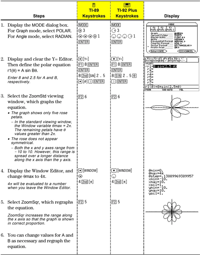
The graph of the polar equation A sin Bθ forms the shape of a rose. Graph the rose for A=8 and B=2.5. Then explore the appearance of the rose for other values of A and B.
| Steps | TI-89 Keystrokes | TI-92 Plus Keystrokes | Display |
|---|---|---|---|
| 1. Display the MODE dialog box.For Graph mode, select POLAR.For Angle mode, select RADIAN. | [MODE]○ 3▽ ▽ ▽ ▶ 1[ENTER] | [MODE]○ 3▽ ▽ ▽ ▶ 1[ENTER] | |
| 2. Display and clear the Y= Editor.Then define the polar equation r1(θ) = A sin Bθ.Enter 8 and 2.5 for A and B, respectively. | ◆ [Y=][F1] 8 [ENTER][ENTER]8 [2nd] [SIN] 2 . 5◆ [θ] ) [ENTER] | ◆ [Y=][F1] 8 [ENTER][ENTER]8 [SIN] 2 . 5 [θ]) [ENTER] | |
| 3. Select the ZoomStd viewing window, which graphs the equation.• The graph shows only five rose petals.– In the standard viewing window, the Window variable θmax = 2π. The remaining petals have θ values greater than 2π.• The rose does not appear symmetrical.– Both the x and y axes range from –10 to 10. However, this range is spread over a longer distance along the x axis than the y axis. | [F2] 6 | [F2] 6 | |
| 4. Display the Window Editor, and change θmax to 4π.4π will be evaluated to a number when you leave the Window Editor. | ◆ [WINDOW]▽4 [2nd] [π] | ◆ [WINDOW]▽4 [2nd] [π] | |
| 5. Select ZoomSqr, which regraphs the equation.ZoomSqr increases the range along the x axis so that the graph is shown in correct proportion. | [F2] 5 | [F2] 5 | |
| 6. You can change values for A and B as necessary and regraph the equation. |
134 Chapter 8: Polar Graphing
Overview of Steps in Graphing Polar Equations
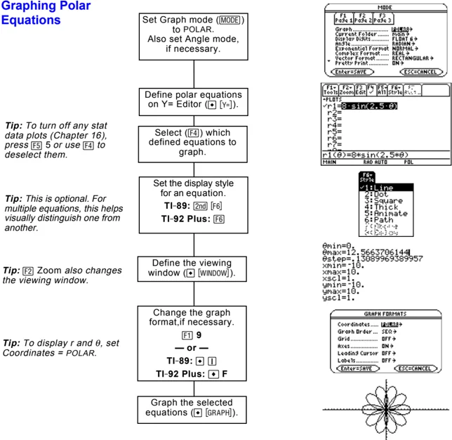
To graph polar equations, use the same general steps used for y(x) functions as described in Chapter 6: Basic Function Graphing. Any differences that apply to polar equations are described on the following pages.
Graphing Polar Equations
Set Graph mode (MODE) to POLAR. Also set Angle mode, if necessary.
Define polar equations on Y= Editor ( [Y=] ).
Tip: To turn off any stat data plots (Chapter 16), press F5 or use F4 to deselect them.
Select (F4) which defined equations to graph.
Set the display style for an equation. TI-89: 2nd F6 TI-92 Plus: F6
Tip: This is optional. For multiple equations, this helps visually distinguish one from another.
Define the viewing window ( WINDOW).
Tip: F2 Zoom also changes the viewing window.
Change the graph format, if necessary. F1 9 — or — TI-89: [ ] [ ] TI-92 Plus: [•] F
Tip: To display r and θ, set Coordinates = POLAR.
Graph the selected equations ( [GRAPH] ).
Exploring the Graph
From the Graph screen, you can:
- Display the coordinates of any pixel by using the free-moving cursor, or of a plotted point by tracing a polar equation.
- Use the F2 Zoom toolbar menu to zoom in or out on a portion of the graph.
- Use the F5 Math toolbar menu to find derivatives, tangents, etc. Some menu items are not available for polar graphs.
Chapter 8: Polar Graphing 135
Differences in Polar and Function Graphing
This chapter assumes that you already know how to graph y(x) functions as described in Chapter 6: Basic Function Graphing. This section describes the differences that apply to polar equations.
Setting the Graph Mode
Use MODE to set Graph = POLAR before you define equations or set Window variables. The Y= Editor and the Window Editor let you enter information for the current Graph mode setting only.
You should also set the Angle mode to the units (RADIAN or DEGREE) you want to use for \theta.
Defining Polar Equations on the Y= Editor
 Tip: You can use the Define command from the Home screen (see Appendix A) to define functions and equations for any graphing mode, regardless of the current mode.
You can define polar equations for r1(\theta) through r99(\theta).
The Y= Editor maintains an independent function list for each Graph mode setting. For example, suppose:
- In FUNCTION graphing mode, you define a set of y(x) functions. You change to POLAR graphing mode and define a set of r(\theta) equations.
- When you return to FUNCTION graphing mode, your y(x) functions are still defined in the Y= Editor. When you return to POLAR graphing mode, your r(\theta) equations are still defined.
Selecting the Display Style
The Above and Below styles are not available for polar equations and are dimmed on the Y= Editor's Style toolbar menu.
136 Chapter 8: Polar Graphing
Window Variables
The Window Editor maintains an independent set of Window variables for each Graph mode setting (just as the Y= Editor maintains independent function lists). Polar graphs use the following Window variables.
Note: You can use a negative θstep. If so, θmin must be greater than θmax.
Standard values (set when you select 6:ZoomStd from the F2 Zoom toolbar menu) are:
θmin = 0.
xmin = -10.
ymin = -10.
θmax = 2π (6.2831853... radians or 360 degrees)
xmax = 10.
ymax = 10.
θstep = π/24 (.1308996... radians or 7.5 degrees)
xscl = 1.
yscl = 1.
You may need to change the standard values for the θ variables (θmin, θmax, θstep) to ensure that enough points are plotted.
Setting the Graph Format
To display coordinates as r and θ values, use:
F1 9
— or —
TI-89: [icon] 1
TI-92 Plus: [icon] F
to set Coordinates = POLAR. If Coordinates = RECT, the polar equations will be graphed properly, but coordinates will be displayed as x and y.
When you trace a polar equation, the θ coordinate is shown even if Coordinates = RECT.
Chapter 8: Polar Graphing 137
Exploring a Graph
As in function graphing, you can explore a graph by using the following tools. Any displayed coordinates are shown in polar or rectangular form as set in the graph format.
\begin{tabular}{ll} \textbf{Tool} & \textbf{For Polar Graphs:} \ Free-Moving Cursor & Works just as it does for function graphs. \ F2 Zoom & Works just as it does for function graphs. \ & \bullet Only x (xmin, xmax, xscl) and y (ymin, ymax, yscl) Window variables are affected. \ & \bullet The \theta Window variables (\thetamin, \thetamax, \thetastep) are not affected unless you select 6:ZoomStd (which sets \thetamin = 0, \thetamax = 2\pi, and \thetastep = \pi/24). \ Tip: During a trace, you can also evaluate r(\theta) by typing the \theta value and pressing ENTER. & F3 Trace Lets you move the cursor along a graph one \thetastep at a time. \ & \bullet When you begin a trace, the cursor is on the first selected equation at \thetamin. \ & \bullet QuickCenter applies to all directions. If you move the cursor off the screen (top or bottom, left or right), press ENTER to center the viewing window on the cursor location. \ & \bullet Automatic panning is not available. If you move the cursor off the left or right side of the screen, the TI-89 / TI-92 Plus will not automatically pan the viewing window. However, you can use QuickCenter. \ Tip: You can use QuickCenter at any time during a trace, even if the cursor is still on the screen. & F5 Math Only 1:Value, 6:Derivatives, 9:Distance, A:Tangent, and B:Arc are available for polar graphs. These tools are based on \theta values. For example: \ & \bullet 1:Value displays an r value (or x and y, depending on the graph format) for a specified \theta value. \ & \bullet 6:Derivatives finds dy/dx or dr/d\theta at a point defined for a specified \theta value. \ \end{tabular}
138 Chapter 8: Polar Graphing
Sequence Graphing
- Preview of Sequence Graphing ........ 140
- Overview of Steps in Graphing Sequences ........ 141
- Differences in Sequence and Function Graphing ........ 142
- Setting Axes for Time, Web, or Custom Plots ........ 146
- Using Web Plots ........ 147
- Using Custom Plots ........ 150
- Using a Sequence to Generate a Table ........ 151
This chapter describes how to graph sequences on the
TI-89 / TI-92 Plus. Before using this chapter, you should be familiar
with Chapter 6: Basic Function Graphing.
Sequences are evaluated only at consecutive integer values. The
two general types of sequences are:
-
Nonrecursive — The nth term in the sequence is a function
of the independent variable n.Each term is independent of any other terms. In the following
example sequence, you can calculate u(5) directly, without
first calculating u(1) or any other previous term.u(n) = 2 * n for n = 1, 2, 3, ...
n is always a series of
consecutive integers,
starting at any positive
integer or zero.u(n) = 2 * n gives the sequence 2, 4, 6, 8, 10, ...
-
Recursive — The nth term is defined in relation to one or
more previous terms, represented by u(n− 1), u(n− 2), etc. In
addition to previous terms, a recursive sequence may also be
defined in relation to n (such as u(n) = u(n− 1) + n).In the following example sequence, you cannot calculate u(5)
without first calculating u(1), u(2), u(3), and u(4).u(n) = 2 * u(n− 1) for n = 1, 2, 3, ...
The first term is undefined
since it has no previous term.
So you must specify an initial
value to use for the first term.Using an initial value of 1:
u(n) = 2 * u(n− 1) gives the sequence 1, 2, 4, 8, 16, ...
The number of initial values you need to specify depends on
how deep the recursion goes. For example, if each term is
defined in relation to the previous two terms, you must specify
initial values for the first two terms.
Note: A recursive sequence
can reference another
sequence. For example,
u2(n) = n² +u1(n− 1).
Chapter 9: Sequence Graphing 139
Preview of Sequence Graphing
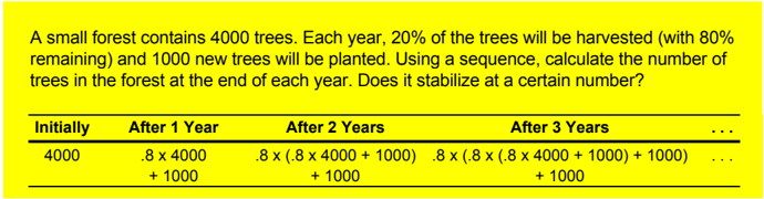
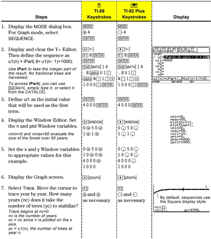
A small forest contains 4000 trees. Each year, 20% of the trees will be harvested (with 80% remaining) and 1000 new trees will be planted. Using a sequence, calculate the number of trees in the forest at the end of each year. Does it stabilize at a certain number?
| Initially | After 1 Year | After 2 Years | After 3 Years | ... |
|---|---|---|---|---|
| 4000 | .8 x 4000+ 1000 | .8 x (.8 x 4000 + 1000)+ 1000 | .8 x (.8 x (.8 x 4000 + 1000) + 1000)+ 1000 | ... |
| Steps | TI-89 Keystrokes | TI-92 Plus Keystrokes | Display |
|---|---|---|---|
| 1. Display the MODE dialog box.For Graph mode, select SEQUENCE. | MODE► 4ENTER | MODE► 4ENTER | |
| 2. Display and clear the Y= Editor.Then define the sequence as u1(n) = iPart(.8* u1(n− 1)+1000).Use iPart to take the integer part of the result. No fractional trees are harvested.To access iPart(, you can use 2nd [MATH], simply type it, or select it from the CATALOG. | ◆ [Y=]F1 8 ENTERENTER2nd [MATH] 1 4. 8 alpha U 1 (□alpha N − 1 ) +1 0 0 0 ) ENTER | ◆ [Y=]F1 8 ENTERENTER2nd [MATH] 1 4. 8 U 1 (□N − 1 ) +1 0 0 0 ) ENTER | |
| 3. Define u1 as the initial value that will be used as the first term. | ENTER4 0 0 0 ENTER | ENTER4 0 0 0 ENTER | |
| 4. Display the Window Editor. Set the n and plot Window variables.nmin=0 and nmax=50 evaluate the size of the forest over 50 years. | ◆ [WINDOW]0 ◄ 5 0 ◄1 ◄ 1 ◄ | ◆ [WINDOW]0 ◄ 5 0 ◄1 ◄ 1 ◄ | nmin=0,nmax=50,plotStrt=1,plotStep=1,xmin=0,xmax=50,xsc1=10,ymin=0,ymax=6000,ysc1=1000. |
| 5. Set the x and y Window variables to appropriate values for this example. | 0 ◄ 5 0 ◄1 0 ◄ 0 ◄6 0 0 0 ◄1 0 0 0 | 0 ◄ 5 0 ◄1 0 ◄ 0 ◄6 0 0 0 ◄1 0 0 0 | |
| 6. Display the Graph screen. | ◆ [GRAPH] | ◆ [GRAPH] | |
| 7. Select Trace. Move the cursor to trace year by year. How many years (nc) does it take the number of trees (yc) to stabilize?Trace begins at nc=0.nc is the number of years.xc = nc since n is plotted on the x axis.yc = u1(n), the number of trees at year n. | F3► and ◄as necessary | F3► and ◄as necessary |
140 Chapter 9: Sequence Graphing
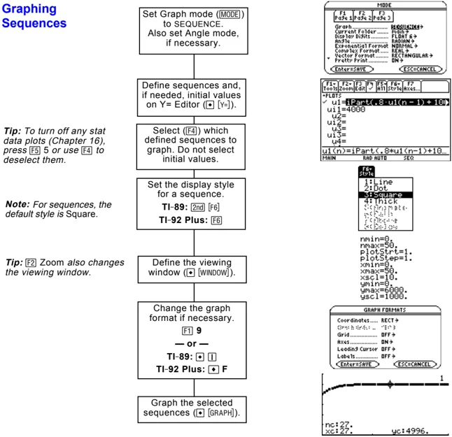
Overview of Steps in Graphing Sequences
To graph sequences, use the same general steps used for y(x) functions as described in Chapter 6: Basic Function Graphing. Any differences are described on the following pages.
Graphing Sequences
Tip: To turn off any stat data plots (Chapter 16), press \boxedF5 5 or use \boxedF4 to deselect them.
Note: For sequences, the default style is Square.
Tip: \boxedF2 Zoom also changes the viewing window.
Tip: You can also evaluate a sequence while tracing. Simply enter the n value directly from the keyboard.
Set Graph mode (\boxedMODE) to SEQUENCE. Also set Angle mode, if necessary.
Define sequences and, if needed, initial values on Y= Editor (\boxedY=).
Select (\boxedF4) which defined sequences to graph. Do not select initial values.
Set the display style for a sequence. TI-89: \boxed2nd \boxedF6 TI-92 Plus: \boxedF6
Define the viewing window (\boxedWINDOW).
Change the graph format if necessary. \boxedF1 9 — or — TI-89: \boxedD \boxedI TI-92 Plus: \boxedD F
Graph the selected sequences (\boxedGRAPH).
Exploring the Graph
From the Graph screen, you can:
- Display the coordinates of any pixel by using the free-moving cursor, or of a plotted point by tracing a sequence.
- Use the \boxedF2 Zoom toolbar menu to zoom in or out on a portion of the graph.
- Use the \boxedF5 Math toolbar menu to evaluate a sequence. Only 1:Value is available for sequences.
- Plot sequences on Time (the default), Web, or Custom axes.
Chapter 9: Sequence Graphing 141
Differences in Sequence and Function Graphing
This chapter assumes that you already know how to graph y(x) functions as described in Chapter 6: Basic Function Graphing. This section describes the differences that apply to sequences.
Setting the Graph Mode
Use MODE to set Graph = SEQUENCE before you define sequences or set Window variables. The Y= Editor and the Window Editor let you enter information for the current Graph mode setting only.
Defining Sequences on the Y= Editor
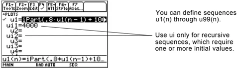
You can define sequences u1(n) through u99(n).
Use ui only for recursive sequences, which require one or more initial values.
Note: You must use a list to enter two or more initial values.
If a sequence requires more than one initial value, enter them as a list enclosed in braces { } and separated by commas.
Enter {1,0} even though {1 0} is shown in the sequence list.
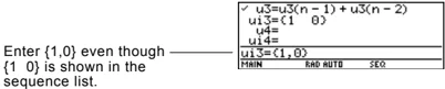
If a sequence requires an initial value but you do not enter one, you will get an error when graphing.
Note: Optionally, for sequences only, you can select different axes for the graph. TIME is the default.
On the Y= Editor, Axes lets you select the axes that are used to graph the sequences. For more detailed information, refer to page 146.
Tip: You can use the Define command from the Home screen (see Appendix A) to define functions and equations for any graphing mode, regardless of the current mode.
The Y= Editor maintains an independent function list for each Graph mode setting. For example, suppose:
• In FUNCTION graphing mode, you define a set of y(x) functions. You change to SEQUENCE graphing mode and define a set of u(n) sequences.
• When you return to FUNCTION graphing mode, your y(x) functions are still defined in the Y= Editor. When you return to SEQUENCE graphing mode, your u(n) sequences are still defined.
142 Chapter 9: Sequence Graphing
Selecting Sequences
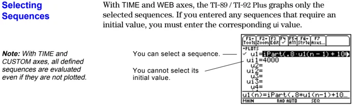
With TIME and WEB axes, the TI-89 / TI-92 Plus graphs only the selected sequences. If you entered any sequences that require an initial value, you must enter the corresponding ui value.
Note: With TIME and CUSTOM axes, all defined sequences are evaluated even if they are not plotted.
You can select a sequence. —— You cannot select its initial value.
With CUSTOM axes, when you specify a sequence in the custom settings, it is graphed regardless of whether it is selected.
Selecting the Display Style
Only the Line, Dot, Square, and Thick styles are available for sequence graphs. Dot and Square mark only those discrete integer values (in plotstep increments) at which a sequence is plotted.
Window Variables
The Window Editor maintains an independent set of Window variables for each Graph mode setting (just as the Y= Editor maintains independent function lists). Sequence graphs use the following Window variables.
| Variable | Description |
|---|---|
| nmin, nmax | Smallest and largest n values to evaluate. Sequences are evaluated at: |
| u(nmin) | |
| u(nmin+1) | |
| u(nmin+2) | |
| ... not to exceed ... | |
| u(nmax) | |
| plotStrt | The term number that will be the first one plotted (depending on plotstep). For example, to begin plotting with the 2nd term in the sequence, set plotstrt = 2. The first term will be evaluated at nmin but not plotted. |
| plotStep | Incremental n value for graphing only. This does not affect how the sequence is evaluated, only which points are plotted. For example, suppose plotstep = 2. The sequence is evaluated at each consecutive integer but is plotted at only every other integer. |
| xmin, xmax, | Boundaries of the viewing window. |
| ymin, ymax | |
| xscl, yscl | Distance between tick marks on the x and y axes. |
Note: Both nmin and nmax must be positive integers, although nmin can be zero.
Note: nmin, nmax, plotstrt and plotstep must be integers ≥ 1. If you do not enter integers, they will be rounded to integers.
Chapter 9: Sequence Graphing 143
Window Variables (Continued)
Standard values (set when you select 6:ZoomStd from the [F2] Zoom toolbar menu) are:
nmin = 1. xmin = -10. ymin = -10. nmax = 10. xmax = 10. ymax = 10. plotStrt = 1. xscl = 1. yscl = 1. plotStep = 1.
You may need to change the standard values for the n and plot variables to ensure that sufficient points are plotted.
To see how plotstrt affects a graph, look at the following examples of a recursive sequence.
Note: Both of these graphs use the same Window variables, except for plotstrt.
This graph is plotted beginning with the 1st term.
 plotStrt=1
This graph is plotted beginning with the 9th term.
 plotStrt=9
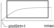
With TIME axes (from Axes on the Y= Editor), you can set plotstrt = 1 and still graph only a selected part of the sequence. Simply define a viewing window that shows only the area of the coordinate plane you want to view.
You could set:
- xmin = first n value to graph
- xmax = nmax (although you can use other values)
- ymin and ymax = expected values for the sequence
 plotStrt=1 nmax
 plotStrt=1 nmax
Changing the Graph Format
The Graph Order format is not available.
- With TIME or CUSTOM axes, multiple sequences are always plotted simultaneously.
- With WEB axes, multiple sequences are always plotted sequentially.
144 Chapter 9: Sequence Graphing
Exploring a Graph
As in function graphing, you can explore a graph by using the following tools. Any displayed coordinates are shown in rectangular or polar form as set in the graph format.
\begin{tabular}{ll} \textbf{Tool} & \textbf{For Sequence Graphs:} \ Free-Moving Cursor & Works just as it does for function graphs. \ F2 Zoom & Works just as it does for function graphs. \ & \begin{itemize} \item Only x (xmin, xmax, xscl) and y (ymin, ymax, ysc1) Window variables are affected. \item The n and plot Window variables (nmin, nmax, plotStrt, plotStep) are not affected unless you select 6:ZoomStd (which sets all Window variables to their standard values). \end{itemize} \ Tip: During a trace, you can evaluate a sequence by typing a value for n and pressing ENTER. & F3 Trace Depending on whether you use TIME, CUSTOM, or WEB axes, Trace operates very differently. \ & \begin{itemize} \item With TIME or CUSTOM axes, you move the cursor along the sequence one plotstep at a time. To move approximately ten plotted points at a time, press \boxed2nd \blacktriangleright or \boxed2nd \blacktriangleleft. \begin{itemize} \item When you begin a trace, the cursor is on the first selected sequence at the term number specified by plotstrt, even if it is outside the viewing window. \item QuickCenter applies to all directions. If you move the cursor off the screen (top or bottom, left or right), press \boxedENTER to center the viewing window on the cursor location. \end{itemize} \item With WEB axes, the trace cursor follows the web, not the sequence. Refer to page 147. \end{itemize} \ Tip: You can use QuickCenter at any time during a trace, even if the cursor is still on the screen. & F5 Math Only 1:Value is available for sequence graphs. \ & \begin{itemize} \item With TIME and WEB axes, the u(n) value (represented by yc) is displayed for a specified n value. \item With CUSTOM axes, the values that correspond to x and y depend on the axes you choose. \end{itemize} \ \end{tabular}
Chapter 9: Sequence Graphing 145
Setting Axes for Time, Web, or Custom Plots
For sequences only, you can select different types of axes for the graph. Examples of the different types are given later in this chapter.
Displaying the AXES Dialog Box
From the Y= Editor, Axes:
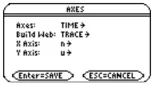
- Depending on the current Axes setting, some items may be dimmed.
- To exit without making any changes, press [ESC].
| Item | Description |
|---|---|
| Axes | TIME — Plots u(n) on the y axis and n on the x axis.WEB — Plots u(n) on the y axis and u(n-1) on the x axis.CUSTOM — Lets you select the x and y axes. |
| Build Web | Active only when Axes = WEB, this specifies whether a web is drawn manually (TRACE) or automatically (AUTO).Refer to page 147 for more information. |
| X Axis and Y Axis | Active only when Axes = CUSTOM, these let you select the value or sequence to plot on the x and y axes.Refer to page 150 for more information. |
To change any of these settings, use the same procedure that you use to change other types of dialog boxes, such as the MODE dialog box.
146 Chapter 9: Sequence Graphing
Using Web Plots
A web plot graphs u(n) vs. u(n− 1), which lets you study the long-term behavior of a recursive sequence. The examples in this section also show how the initial value can affect a sequence's behavior.
Valid Functions for Web Plots
A sequence must meet the following criteria; otherwise, it will not be graphed properly on WEB axes. The sequence:
- Must be recursive with only one recursion level; u(n− 1) but not u(n− 2).
- Cannot reference n directly.
- Cannot reference any other defined sequence except itself.
When You Display the Graph Screen
After you select WEB axes and display the Graph screen, the TI-89 / TI-92 Plus:
- Draws a y=x reference line.
- Plots the selected sequence definitions as functions, with u(n− 1) as the independent variable. This effectively converts a recursive sequence into a nonrecursive form for graphing.
For example, consider the sequence u1(n) = \sqrt5-u1(n-1) and an initial value of ui1=1. The TI-89 / TI-92 Plus draws the y=x reference line and then plots y = \sqrt5-x.
Drawing the Web
After the sequence is plotted, the web may be displayed manually or automatically, depending on how you set Build Web on the AXES dialog box.
\begin{tabular}{ll} If Build Web = & The web is: \ TRACE & Not drawn until you press F3. The web is then drawn step-by-step as you move the trace cursor (you must have an initial value before using Trace). \ & Note: With WEB axes, you cannot trace along the sequence itself as you do in other graphing modes. \ AUTO & Drawn automatically. You can then press F3 to trace the web and display its coordinates. \ \end{tabular}
The web:
- Starts on the x axis at the initial value ui (when plotstrt = 1).
- Moves vertically (either up or down) to the sequence.
- Moves horizontally to the y=x reference line.
- Repeats this vertical and horizontal movement until n=nmax.
Note: The web starts at plotstrt. The value of n is incremented by 1 each time the web moves to the sequence (plotStep is ignored).
Chapter 9: Sequence Graphing 147
Example: Convergence
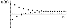
- On the Y= Editor ( [Y=] ), define u1(n) = -.8u1(n-1) + 3.6. Set initial value ui1 = -4.
- Set Axes = TIME.
- On the Window Editor ([WINDOW]), set the Window variables. nmin=1. xmin=0. ymin=-10. nmax=25. xmax=25. ymax=10. plotStrt=1. xscl=1. yscl=1. plotstep=1.
- Graph the sequence ([GRAPH]).
By default, a sequence uses the Square display style.
- On the Y= Editor, set Axes = WEB and Build Web = AUTO.
- On the Window Editor, change the Window variables. nmin=1. xmin=-10. ymin=-10. nmax=25. xmax=10. ymax=10. plotStrt=1. xscl=1. yscl=1. plotStep=1.
- Repgraph the sequence.
Web plots are always shown as lines, regardless of the selected display style.
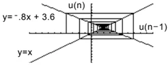
- Press F3. As you press \blacklozenge, the trace cursor follows the web. The screen displays the cursor coordinates nc, xc, and yc (where xc and yc represent u(n-1) and u(n), respectively).
As you trace to larger values of nc, you can see xc and yc approach the convergence point.
Tip: During a trace, you can move the cursor to a specified n value by typing the value and pressing ENTER.
Tip: When the nc value changes, the cursor is on the sequence. The next time you press \blacklozenge, nc stays the same but the cursor is now on the y=x reference line.
Example: Divergence
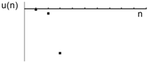
- On the Y= Editor ( [Y=] ), define u1(n) = 3.2u1(n-1) -.8(u1(n-1))$^2$. Set initial value ui1 = 4.45.
- Set Axes = TIME.
- On the Window Editor ([WINDOW]), set the Window variables. nmin=0. xmin=0. ymin=-75. nmax=10. xmax=10. ymax=10. plotStrt=1. xscl=1. yscl=1. plotStep=1.
- Graph the sequence ([GRAPH]).
Because the sequence quickly diverges to large negative values, only a few points are plotted.
148 Chapter 9: Sequence Graphing
-
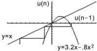
On the Y= Editor, set Axes = WEB and Build Web = AUTO.
-
On the Window Editor, change the Window variables. nmin=0. xmin= -10. ymin= -10. nmax=10. xmax=10. ymax=10. plotStrt=1. xscl=1. yscl=1. plotStep=1.
-
Repgraph the sequence. The web plot shows how quickly the sequence diverges to large negative values.
Example: Oscillation
This example shows how the initial value can affect a sequence.
-
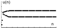
On the Y= Editor ( [Y=] ), use the same sequence defined in the divergence example: u1(n) = 3.2u1(n-1) – .8(u1(n-1))². Set initial value ui1 = 0.5.
-
Set Axes = TIME.
-
On the Window Editor ([WINDOW]), set the Window variables. nmin=1. xmin=0. ymin=0. nmax=100. xmax=100. ymax=5. plotStrt=1. xscl=10. yscl=1. plotStep=1.
-
Graph the sequence ([GRAPH]). Note: Compare this graph with the divergence example. This is the same sequence with a different initial value.
-
On the Y= Editor, set Axes = WEB and Build Web = AUTO.
-
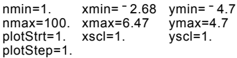
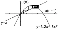
On the Window Editor, change the Window variables. nmin=1. xmin= -2.68 ymin= -4.7 nmax=100. xmax=6.47 ymax=4.7 plotStrt=1. xscl=1. yscl=1. plotStep=1.
-
Repgraph the sequence. Note: The web moves to an orbit oscillating between two stable points.
-
Press F3. Then use \diamond to trace the web. As you trace to larger values of n, notice that xc and yc oscillate between 2.05218 and 3.19782.
-
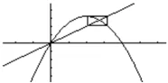
On the Window Editor, set plotstrt=50. Then regraph the sequence. Note: By starting the web plot at a later term, the stable oscillation orbit is shown more clearly.
Chapter 9: Sequence Graphing 149
Using Custom Plots
CUSTOM axes give you great flexibility in graphing sequences. As shown in the following example, CUSTOM axes are particularly effective for showing relationships between one sequence and another.
Example: Predator-Prey Model
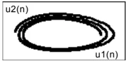
Using the predator-prey model in biology, determine the numbers of rabbits and foxes that maintain population equilibrium in a certain region.
R = Number of rabbits M = Growth rate of rabbits if there are no foxes (use .05) K = Rate at which foxes can kill rabbits (use .001) W = Number of foxes G = Growth rate of foxes if there are rabbits (use .0002) D = Death rate of foxes if there are no rabbits (use .03)
$R_n = R_{n-1} (1 + M - K W_{n-1})$ $W_n = W_{n-1} (1 + G R_{n-1} - D)$
Note: Assume there are initially 200 rabbits and 50 foxes.
-
On the Y= Editor ([Y=]), define the sequences and initial values for $R_n$ and $W_n$. u1(n) = u1(n- 1) * (1 + .05 -.001 * u2(n- 1)) ui1 = 200 u2(n) = u2(n- 1) * (1 + .0002 * u1(n- 1) -.03) ui2 = 50
-
Set Axes = TIME.
-
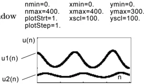
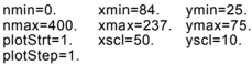
On the Window Editor ([WINDOW]), set the Window variables. nmin=0. xmin=0. ymin=0. nmax=400. xmax=400. ymax=300. plotStrt=1. xscl=100. yscl=100. plotStep=1.
Note: Use F3 to individually trace the number of rabbits u1(n) and foxes u2(n) over time (n).
- Graph the sequence ([GRAPH]).
-
On the Y= Editor, set Axes = CUSTOM, X Axis = u1, and Y Axis = u2.
-
In the Window Editor, change the Window variables. nmin=0. xmin=84. ymin=25. nmax=400. xmax=237. ymax=75. plotStrt=1. xscl=50. yscl=10. plotStep=1.
Note: Use F3 to trace both the number of rabbits (xc) and foxes (yc) over the cycle of 400 generations.
- Regraph the sequence.
150 Chapter 9: Sequence Graphing
Using a Sequence to Generate a Table
Previous sections described how to graph a sequence. You can also use a sequence to generate a table. Refer to Chapter 13 for detailed information about tables.
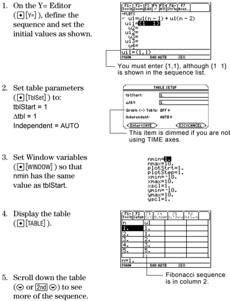
Example: Fibonacci Sequence
In a Fibonacci sequence, the first two terms are 1 and 1. Each succeeding term is the sum of the two immediately preceding terms.
- On the Y= Editor ( [Y=] ), define the sequence and set the initial values as shown.
You must enter {1,1}, although {1 1} is shown in the sequence list.
- Set table parameters ( [TblSet] ) to: tblStart = 1 Δtbl = 1 Independent = AUTO
This item is dimmed if you are not using TIME axes.
- Set Window variables ( [WINDOW] ) so that nmin has the same value as tblStart.
nmin=1 nmax=10. PlotStart=1. PlotStep=1. xmin=-10. xmax=10. xscale=1. ymin=-10. ymax=10. yscl=1.
- Display the table ( [TABLE] ).
Fibonacci sequence is in column 2.
- Scroll down the table ( or [2nd] ) to see more of the sequence.
Chapter 9: Sequence Graphing 151
152 Chapter 9: Sequence Graphing
3D Graphing
10
- Preview of 3D Graphing ........ 154
- Overview of Steps in Graphing 3D Equations ........ 156
- Differences in 3D and Function Graphing ........ 157
- Moving the Cursor in 3D ........ 160
- Rotating and/or Elevating the Viewing Angle ........ 162
- Animating a 3D Graph Interactively ........ 164
- Changing the Axes and Style Formats ........ 165
- Contour Plots ........ 167
- Example: Contours of a Complex Modulus Surface ........ 170
- Implicit Plots ........ 171
- Example: Implicit Plot of a More Complicated Equation ........ 173
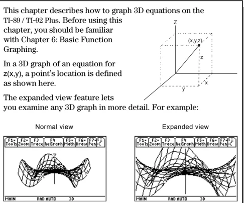
This chapter describes how to graph 3D equations on the TI-89 / TI-92 Plus. Before using this chapter, you should be familiar with Chapter 6: Basic Function Graphing.
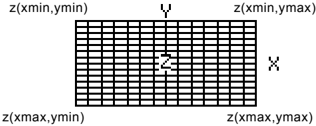
In a 3D graph of an equation for z(x,y), a point's location is defined as shown here.
The expanded view feature lets you examine any 3D graph in more detail. For example:

Tip: To view the graph along the x, y, or z axis, you can press X, Y, or Z, respectively.
Tip: To switch from one format style to the next (skipping IMPLICIT PLOT), press: TI-89: [alpha] [F] TI-92 Plus: F.
This retains the current view (either expanded or normal).
Note: To switch to IMPLICIT PLOT (via the GRAPH FORMATS dialog box), press: TI-89: [◄] [1] TI-92 Plus: [►] F.
To switch between normal and expanded views, press [×] (multiplication key, not the letter X).
When you display a 3D graph, the expanded view is used automatically if:
- You set or change the graph format style to CONTOUR LEVELS or IMPLICIT PLOT.
- The previous graph used the expanded view.
If you press a cursor key to animate the graph, the screen switches to the normal view automatically. You cannot animate a graph in the expanded view.
Chapter 10: 3D Graphing 153

Preview of 3D Graphing
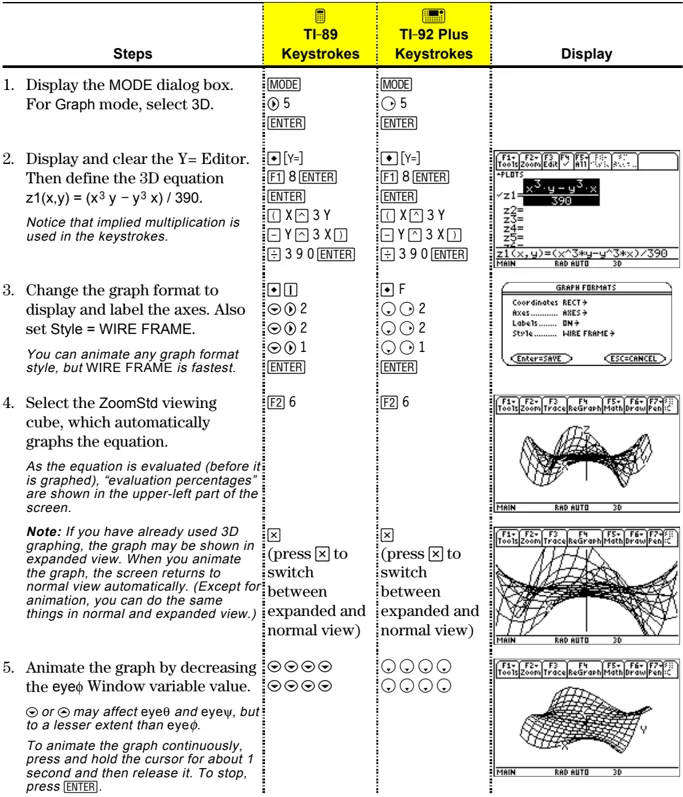
Graph the 3D equation z(x,y) = (x³ y – y³ x) / 390. Animate the graph by using the cursor to interactively change the eye Window variable values that control your viewing angle. Then view the graph in different graph format styles.
| Steps | TI-89 Keystrokes | TI-92 Plus Keystrokes | Display |
|---|---|---|---|
| 1. Display the MODE dialog box. For Graph mode, select 3D. | MODE► 5ENTER |
MODE► 5ENTER |
|
| 2. Display and clear the Y= Editor. Then define the 3D equation z1(x,y) = (x³ y – y³ x) / 390.Notice that implied multiplication is used in the keystrokes. | ♦ [Y=]F1 8 ENTERENTER□ X ^ 3 Y– Y ^ 3 X □÷ 3 9 0 ENTER |
♦ [Y=]F1 8 ENTERENTER□ X ^ 3 Y– Y ^ 3 X □÷ 3 9 0 ENTER |
|
| 3. Change the graph format to display and label the axes. Also set Style = WIRE FRAME.You can animate any graph format style, but WIRE FRAME is fastest. | ♦ I▼ ► 2▼ ► 2▼ ► 1ENTER |
♦ F▼ ► 2▼ ► 2▼ ► 1ENTER |
|
| 4. Select the ZoomStd viewing cube, which automatically graphs the equation.As the equation is evaluated (before it is graphed), “evaluation percentages” are shown in the upper-left part of the screen.Note: If you have already used 3D graphing, the graph may be shown in expanded view. When you animate the graph, the screen returns to normal view automatically. (Except for animation, you can do the same things in normal and expanded view.) | F2 6×(press × to switch between expanded and normal view) |
F2 6×(press × to switch between expanded and normal view) |
|
5. Animate the graph by decreasing the eyeφ Window variable value.▶ or ◀ may affect eyeθ and eyeψ, but to a lesser extent than eyeφ.To animate the graph continuously, press and hold the cursor for about 1 second and then release it. To stop, press ENTER. |
▼ ▼ ▼ ▼▼ ▼ ▼ ▼ |
▼ ▼ ▼ ▼▼ ▼ ▼ ▼ |
154 Chapter 10: 3D Graphing
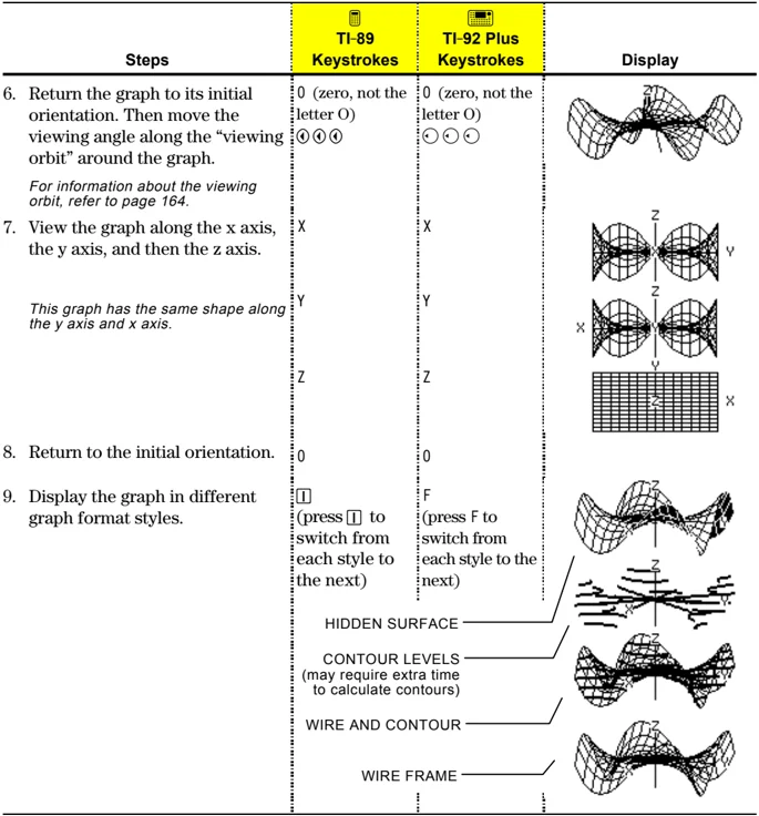
\begin{tabular}{|p{0.3\textwidth}|p{0.2\textwidth}|p{0.2\textwidth}|p{0.2\textwidth}|} \hline \textbf{Steps} & \textbf{TI-89 Keystrokes} & \textbf{TI-92 Plus Keystrokes} & \textbf{Display} \ \hline 6. Return the graph to its initial orientation. Then move the viewing angle along the "viewing orbit" around the graph.
For information about the viewing orbit, refer to page 164. & 0 (zero, not the letter O) \circlearrowleft \circlearrowleft \circlearrowleft & 0 (zero, not the letter O) \circlearrowleft \circlearrowleft \circlearrowleft & \ \hline 7. View the graph along the x axis, the y axis, and then the z axis.
This graph has the same shape along the y axis and x axis. & X & X & \ & Y & Y & \ & Z & Z & \ \hline 8. Return to the initial orientation. & 0 & 0 & \ \hline 9. Display the graph in different graph format styles. & F (press F to switch from each style to the next) & F (press F to switch from each style to the next) & HIDDEN SURFACE \ & & & CONTOUR LEVELS (may require extra time to calculate contours) \ & & & WIRE AND CONTOUR \ & & & WIRE FRAME \ \hline \end{tabular}
Note: You can also display the graph as an implicit plot by using the GRAPH FORMATS dialog box (\fboxF1 9 or TI-89: \fboxD \fboxF1 TI-92 Plus: \fboxD F). If you press TI-89: \fboxF1 TI-92 Plus: F to switch between styles, the implicit plot is not displayed.
Chapter 10: 3D Graphing 155
Overview of Steps in Graphing 3D Equations
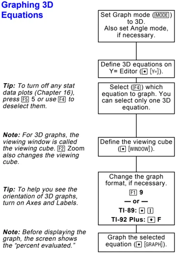
To graph 3D equations, use the same general steps used for y(x) functions as described in Chapter 6: Basic Function Graphing. Any differences that apply to 3D equations are described on the following pages.
Graphing 3D Equations
Tip: To turn off any stat data plots (Chapter 16), press F5 or use F4 to deselect them.
Set Graph mode (MODE) to 3D. Also set Angle mode, if necessary.
Define 3D equations on Y= Editor ( [ZOOM] [Y=] ).
Select ([F4]) which equation to graph. You can select only one 3D equation.
Note: For 3D graphs, the viewing window is called the viewing cube. [F2] Zoom also changes the viewing cube.
Define the viewing cube ([ZOOM] [WINDOW]).
eyeθ=20. eyeφ=70. eleφ=0. xmin=-10. xmax=10. xgrid=4. ymin=-10. ymax=10. ygrid=4. zmin=-10. zmax=10. ncontour=5.
Tip: To help you see the orientation of 3D graphs, turn on Axes and Labels.
Change the graph format, if necessary. [F1] 9 — or — TI-89: [ZOOM] [1] TI-92 Plus: [ZOOM] F
Note: Before displaying the graph, the screen shows the "percent evaluated."
Graph the selected equation ([ZOOM] [GRAPH]).
Exploring the Graph
Tip: You can also evaluate z(x,y) while tracing. Type the x value and press [ENTER]; then type the y value and press [ENTER].
From the Graph screen, you can:
- Trace the equation.
- Use the [F2] Zoom toolbar menu to zoom in or out on a portion of the graph. Some of the menu items are dimmed because they are not available for 3D graphs.
- Use the [F5] Math toolbar menu to evaluate the equation at a specified point. Only 1:Value is available for 3D graphs.
156 Chapter 10: 3D Graphing
Differences in 3D and Function Graphing
This chapter assumes that you already know how to graph y(x) functions as described in Chapter 6: Basic Function Graphing. This section describes the differences that apply to 3D equations.
Setting the Graph Mode
Use MODE to set Graph = 3D before you define equations or set Window variables. The Y= Editor and the Window Editor let you enter information for the current Graph mode setting only.
Defining 3D Equations on the Y= Editor
 You can define 3D equations for z1(x,y) through z99(x,y).
Tip: You can use the Define command from the Home screen (see Appendix A) to define functions and equations for any graphing mode, regardless of the current mode.
The Y= Editor maintains an independent function list for each Graph mode setting. For example, suppose:
- In FUNCTION graphing mode, you define a set of y(x) functions. You change to 3D graphing mode and define a set of z(x,y) equations.
- When you return to FUNCTION graphing mode, your y(x) functions are still defined in the Y= Editor. When you return to 3D graphing mode, your z(x,y) equations are still defined.
Selecting the Display Style
Because you can graph only one 3D equation at a time, display styles are not available. On the Y= Editor, Style toolbar menu is dimmed.
For 3D equations, however, you can use:
F1 9 — or — TI-89: [diamond] 1 TI-92 Plus: [diamond] F
to set the Style format to WIRE FRAME or HIDDEN SURFACE. Refer to “Changing the Axes and Style Formats” on page 165.
Chapter 10: 3D Graphing 157
Window Variables
The Window Editor maintains an independent set of Window variables for each Graph mode setting (just as the Y= Editor maintains independent function lists). 3D graphs use the following Window variables.
\begin{tabular}{ll} \hline Variable & Description \ \hline eye\theta, eye\phi, & Angles (always in degrees) used to view the graph. \ eye\psi & Refer to "Rotating and/or Elevating the Viewing Angle" \ & on page 162. \ xmin, xmax, & Boundaries of the viewing cube. \ ymin, ymax, & \ zmin, zmax & \ xgrid, ygrid & The distance between xmin and xmax and between ymin \ & and ymax is divided into the specified number of grids. \ & The z(x,y) equation is evaluated at each grid point \ & where the grid lines (or grid wires) intersect. \ & The incremental value along x and y is calculated as: \ & x increment = \fracx_max - x_minxgrid \quad y increment = \fracy_max - y_minygrid \ & The number of grid wires is xgrid + 1 and ygrid + 1. For \ & example, when xgrid = 14 and ygrid = 14, the xy grid \ & consists of 225 (15 × 15) grid points. \ ncontour & The number of contours evenly distributed along the \ & displayed range of z values. Refer to page 168. \ \hline \end{tabular}
Note: If you enter a fractional number for xgrid or ygrid, it is rounded to the nearest whole number ≥ 1.
Note: The 3D mode does not have scl Window variables, so you cannot set tick marks on the axes.
Standard values (set when you select 6:ZoomStd from the F2 Zoom toolbar menu) are:
eye\theta = 20. \quad xmin = -10. \quad ymin = -10. \quad zmin = -10. eye\phi = 70. \quad xmax = 10. \quad ymax = 10. \quad zmax = 10. eye\psi = 0. \quad xgrid = 14. \quad ygrid = 14. \quad ncontour = 5.

Note: Increasing the grid variables decreases the graphing speed.
You may need to increase the standard values for the grid variables (xgrid, ygrid) to ensure that enough points are plotted.
158 Chapter 10: 3D Graphing