cos⁻¹()
TI-89: ◻ [cos⁻¹] key
TI-92 Plus: [2nd] [cos⁻¹] key
cos⁻¹(expression1) ⇒ expression
cos⁻¹(list1) ⇒ list
cos⁻¹(expression1) returns the angle whose cosine is expression1 as an expression.
cos⁻¹(list1) returns a list of the inverse cosines of each element of list1.
Note: The result is returned as either a degree or radian angle, according to the current angle mode setting.
In Degree angle mode:
cos⁻¹(1) [ENTER]
0
In Radian angle mode:
cos⁻¹({0,.2,.5}) [ENTER]
{π/2 1.369... 1.047...}
cos⁻¹(squareMatrix1) ⇒ squareMatrix
Returns the matrix inverse cosine of squareMatrix1. This is not the same as calculating the inverse cosine of each element. For information about the calculation method, refer to cos().
squareMatrix1 must be diagonalizable. The result always contains floating-point numbers.
In Radian angle mode and Rectangular complex format mode:
cos⁻¹([1,5,3;4,2,1;6,-2,1]) [ENTER]
[1.734...+.064...·i -1.490...+2.105...·i ...]
[-.725...+1.515...·i .623...+.778...·i ...]
[-2.083...+2.632...·i 1.790...-1.271...·i ...]
cosh()
MATH/Hyperbolic menu
cosh(expression1) ⇒ expression
cosh(list1) ⇒ list
cosh(expression1) returns the hyperbolic cosine of the argument as an expression.
cosh(list1) returns a list of the hyperbolic cosines of each element of list1.
In Radian angle mode:
cosh(1.2) [ENTER]
1.810...
cosh({0,1.2}) [ENTER]
{1 1.810...}
cosh(squareMatrix1) ⇒ squareMatrix
Returns the matrix hyperbolic cosine of squareMatrix1. This is not the same as calculating the hyperbolic cosine of each element. For information about the calculation method, refer to cos().
squareMatrix1 must be diagonalizable. The result always contains floating-point numbers.
cosh([1,5,3;4,2,1;6,-2,1]) [ENTER]
[421.255 253.909 216.905]
[327.635 255.301 202.958]
[226.297 216.623 167.628]
cosh⁻¹()
MATH/Hyperbolic menu
cosh⁻¹(expression1) ⇒ expression
cosh⁻¹(list1) ⇒ list
cosh⁻¹(expression1) returns the inverse hyperbolic cosine of the argument as an expression.
cosh⁻¹(list1) returns a list of the inverse hyperbolic cosines of each element of list1.
cosh⁻¹(1) [ENTER]
0
cosh⁻¹({1,2.1,3}) [ENTER]
{0 1.372... cosh⁻¹(3)}
424 Appendix A: Functions and Instructions
cosh⁻¹(squareMatrix1) ⇒ squareMatrix
Returns the matrix inverse hyperbolic cosine of squareMatrix1. This is not the same as calculating the inverse hyperbolic cosine of each element. For information about the calculation method, refer to cos().
squareMatrix1 must be diagonalizable. The result always contains floating-point numbers.
In Radian angle mode and Rectangular complex format mode:
cosh⁻¹([1,5,3;4,2,1;6,-2,1]) [ENTER] [ 2.525...+1.734...·i -0.009...-1.490...·i ... ] [ .486...-.725...·i 1.662...+.623...·i ... ] [ -.322...-2.083...·i 1.267...+1.790...·i ... ]
crossP() MATH/Matrix/Vector ops menu
crossP(list1, list2) ⇒ list
Returns the cross product of list1 and list2 as a list.
list1 and list2 must have equal dimension, and the dimension must be either 2 or 3.
crossP({a1,b1},{a2,b2}) [ENTER] {0 0 a1·b2−a2·b1}
crossP({0.1,2.2,-5},{1,-.5,0}) [ENTER] {-2.5 -5. -2.25}
crossP(vector1, vector2) ⇒ vector
Returns a row or column vector (depending on the arguments) that is the cross product of vector1 and vector2.
Both vector1 and vector2 must be row vectors, or both must be column vectors. Both vectors must have equal dimension, and the dimension must be either 2 or 3.
crossP([1,2,3],[4,5,6]) [ENTER] [-3 6 -3]
crossP([1,2],[3,4]) [ENTER] [0 0 -2]
cSolve() MATH/Algebra/Complex menu
cSolve(equation, var) ⇒ Boolean expression
Returns candidate complex solutions of an equation for var. The goal is to produce candidates for all real and non-real solutions. Even if equation is real, cSolve() allows non-real results in real mode.
Although the TI-89 / TI-92 Plus processes all undefined variables as if they were real, cSolve() can solve polynomial equations for complex solutions.
cSolve() temporarily sets the domain to complex during the solution even if the current domain is real. In the complex domain, fractional powers having odd denominators use the principal rather than the real branch. Consequently, solutions from solve() to equations involving such fractional powers are not necessarily a subset of those from cSolve().
cSolve(x^3=-1,x) [ENTER] solve(x^3=-1,x) [ENTER] ■ cSolve(x³ = -1, x) □/□ + √□/□·i or x = □/□ - √□/□·i ■ solve(x³ = -1, x) x = -1
cSolve(x^(1/3)=-1,x) [ENTER] false solve(x^(1/3)=-1,x) [ENTER] x = -1
Appendix A: Functions and Instructions 425
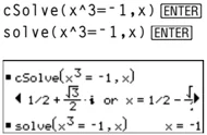
cSolve() starts with exact symbolic methods. Except in EXACT mode, cSolve() also uses iterative approximate complex polynomial factoring, if necessary.
Note: See also cZeros(), solve(), and zeros().
Note: If equation is non-polynomial with functions such as abs(), angle(), conj(), real(), or imag(), you should place an underscore _ (TI-89: [♦] [] TI-92 Plus: [2nd] []) at the end of var. By default, a variable is treated as a real value.
If you use var_, the variable is treated as complex.
You should also use var_ for any other variables in equation that might have unreal values. Otherwise, you may receive unexpected results.
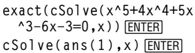
Display Digits mode in Fix 2: exact(cSolve(x^5+4x^4+5x ^3-6x-3=0,x)) [ENTER] cSolve(ans(1),x) [ENTER]
z is treated as real: cSolve(conj(z)=1+i,z) [ENTER] $$z=1+i$$
z_ is treated as complex: cSolve(conj(z_)=1+i,z_) [ENTER] $$z_=1-i$$
cSolve(equation1 and equation2 [and ... ], {varOrGuess1, varOrGuess2 [, ... ]}) \Rightarrow Boolean expression
Returns candidate complex solutions to the simultaneous algebraic equations, where each varOrGuess specifies a variable that you want to solve for.
Optionally, you can specify an initial guess for a variable. Each varOrGuess must have the form:
variable – or – variable = real or non-real number
For example, x is valid and so is x=3+i.
If all of the equations are polynomials and if you do NOT specify any initial guesses, cSolve() uses the lexical Gröbner/Buchberger elimination method to attempt to determine all complex solutions.
Complex solutions can include both real and non-real solutions, as in the example to the right.
Note: The following examples use an underscore _ (TI-89: [♦] [] TI-92 Plus: [2nd] []) so that the variables will be treated as complex.
cSolve(u_*v_-u_=v_ and v_^2=-u_,{u_,v_}) [ENTER]
$u_=1/2 + \frac\sqrt32i and v_=1/2 - \frac\sqrt32i$
or $u_=1/2 - \frac\sqrt32i and v_=1/2 + \frac\sqrt32i$
or $u_=0 and v_=0$
426 Appendix A: Functions and Instructions
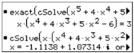
Simultaneous polynomial equations can have extra variables that have no values, but represent given numeric values that could be substituted later.
You can also include solution variables that do not appear in the equations. These solutions show how families of solutions might contain arbitrary constants of the form @k, where k is an integer suffix from 1 through 255. The suffix resets to 1 when you use ClrHome or F1 8:Clear Home.
For polynomial systems, computation time or memory exhaustion may depend strongly on the order in which you list solution variables. If your initial choice exhausts memory or your patience, try rearranging the variables in the equations and/or varOrGuess list.
If you do not include any guesses and if any equation is non-polynomial in any variable but all equations are linear in all solution variables, cSolve() uses Gaussian elimination to attempt to determine all solutions.
If a system is neither polynomial in all of its variables nor linear in its solution variables, cSolve() determines at most one solution using an approximate iterative method. To do so, the number of solution variables must equal the number of equations, and all other variables in the equations must simplify to numbers.
A non-real guess is often necessary to determine a non-real solution. For convergence, a guess might have to be rather close to a solution.
Appendix A: Functions and Instructions 427
CubicReg MATH/Statistics/Regressions menu
CubicReg list1, list2[, [list3] [, list4, list5]]
Calculates the cubic polynomial regression and updates all the statistics variables.
All the lists must have equal dimensions except for list5.
list1 represents xlist.
list2 represents ylist.
list3 represents frequency.
list4 represents category codes.
list5 represents category include list.
Note: list1 through list4 must be a variable name or c1–c99 (columns in the last data variable shown in the Data/Matrix Editor). list5 does not have to be a variable name and cannot be c1–c99.
In function graphing mode.
{0,1,2,3}→L1 ENTER {0 1 2 3}
{0,2,3,4}→L2 ENTER {0 2 3 4}
CubicReg L1,L2 ENTER Done
ShowStat ENTER
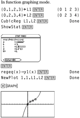
ENTER
regeq(x)→y1(x) ENTER Done
NewPlot 1,1,L1,L2 ENTER Done
♦ [GRAPH]
cumSum() MATH/List menu
cumSum(list1) ⇒ list
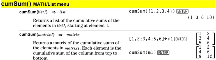
Returns a list of the cumulative sums of the elements in list1, starting at element 1.
cumSum({1,2,3,4}) ENTER {1 3 6 10}
cumSum(matrix1) ⇒ matrix
Returns a matrix of the cumulative sums of the elements in matrix1. Each element is the cumulative sum of the column from top to bottom.
[1,2;3,4;5,6]→m1 ENTER
cumSum(m1) ENTER
\beginbmatrix 1 & 2 \ 3 & 4 \ 5 & 6 \endbmatrix
\beginbmatrix 1 & 2 \ 4 & 6 \ 9 & 12 \endbmatrix
CustmOff CATALOG
CustmOff
Removes a custom toolbar.
CustmOn and CustmOff enable a program to control a custom toolbar. Manually, you can press [2nd][CUSTOM] to toggle a custom toolbar on and off. Also, a custom toolbar is removed automatically when you change applications.
See Custom program listing example.
CustmOn CATALOG
CustmOn
Activates a custom toolbar that has already been set up in a Custom...EndCustm block.
CustmOn and CustmOff enable a program to control a custom toolbar. Manually, you can press [2nd][CUSTOM] to toggle a custom toolbar on and off.
See Custom program listing example.
428 Appendix A: Functions and Instructions
Custom 2nd [CUSTOM] key
Custom block EndCustm
Sets up a toolbar that is activated when you press 2nd [CUSTOM]. It is very similar to the ToolBar instruction except that Title and Item statements cannot have labels.
block can be either a single statement or a series of statements separated with the “:” character.
Note: 2nd [CUSTOM] acts as a toggle. The first instance invokes the menu, and the second instance removes the menu. The menu is removed also when you change applications.
Program listing: :Test( ) :Prgm :Custom :Title "Lists" :Item "List1" :Item "Scores" :Item "L3" :Title "Fractions" :Item "f(x)" :Item "h(x)" :Title "Graph" :EndCustm :EndPrgm
Cycle CATALOG
Cycle
Transfers program control immediately to the next iteration of the current loop (For, While, or Loop).
Cycle is not allowed outside the three looping structures (For, While, or Loop).
Program listing: :● Sum the integers from 1 to 100 skipping 50. :0→temp :For i,1,100,1 :If i=50 :Cycle :temp+i→temp :EndFor :Disp temp
Contents of temp after execution: 5000
CyclePic CATALOG
CyclePic picNameString, n [, [wait], [cycles], [direction]]
Displays all the PIC variables specified and at the specified interval. The user has optional control over the time between pictures, the number of times to cycle through the pictures, and the direction to go, circular or forward and backwards.
direction is 1 for circular or -1 for forward and backwards. Default = 1.
- Save three pics named pic1, pic2, and pic3.
- Enter: CyclePic "pic", 3, .5, 4, -1
- The three pictures (3) will be displayed automatically—one-half second (.5) between pictures, for four cycles (4), and forward and backwards (-1).
►Cy lind MATH/Matrix/Vector ops menu
vector ►Cy lind
[2,2,3] ►Cy lind ENTER
Displays the row or column vector in cylindrical form [r∠θ, z].
vector must have exactly three elements. It can be either a row or a column.
[2√2 ∠ π/4 3]
Appendix A: Functions and Instructions 429
cZeros() MATH/Algebra/Complex menu
cZeros(expression, var) \Rightarrow list
Returns a list of candidate real and non-real values of var that make expression=0. $cZeros()$ does this by computing exp\trianglerightlist(cSolve(expression=0,var),var). Otherwise, $cZeros()$ is similar to $zeros()$.
Note: See also $cSolve()$, $solve()$, and $zeros()$.
Note: If expression is non-polynomial with functions such as $abs()$, $angle()$, $conj()$, $real()$, or $imag()$, you should place an underscore _ (TI-89: \boxed\blacksquare[_]. TI-92 Plus: \boxed2nd[_]) at the end of var. By default, a variable is treated as a real value. If you use var_ , the variable is treated as complex.
You should also use var_ for any other variables in expression that might have unreal values. Otherwise, you may receive unexpected results.
Display Digits mode in Fix 3:
cZeros(x^5+4x^4+5x^3-6x-3,x) ENTER { -2.125 -.612 .965 -1.114-1.073i -1.114+1.073i }
z is treated as real: cZeros(conj(z)-1-i,z) ENTER {1+i}
z_ is treated as complex: cZeros(conj(z_)-1-i,z_) ENTER {1-i}
cZeros(\expression1, expression2 [\dots], \varOrGuess1,varOrGuess2 [\dots]) \Rightarrow matrix
Returns candidate positions where the expressions are zero simultaneously. Each varOrGuess specifies an unknown whose value you seek.
Optionally, you can specify an initial guess for a variable. Each varOrGuess must have the form:
variable – or – variable = real or non-real number
For example, x is valid and so is x=3+$i$.
If all of the expressions are polynomials and you do NOT specify any initial guesses, $cZeros()$ uses the lexical Gröbner/Buchberger elimination method to attempt to determine all complex zeros.
Complex zeros can include both real and non-real zeros, as in the example to the right.
Each row of the resulting matrix represents an alternate zero, with the components ordered the same as the varOrGuess list. To extract a row, index the matrix by [row].
Note: The following examples use an underscore _ (TI-89: \boxed\blacksquare[_]. TI-92 Plus: \boxed2nd[_]) so that the variables will be treated as complex.
cZeros({u_*v_-u_-v_,v_^2+u_}, {u_,v_}) ENTER
$$ \begin{bmatrix} 1/2 & -\frac{\sqrt{3}}{2}i & 1/2 + \frac{\sqrt{3}}{2}i \ 1/2 + \frac{\sqrt{3}}{2}i & 1/2 - \frac{\sqrt{3}}{2}i \ 0 & 0 \end{bmatrix} $$
Extract row 2: ans(1)[2] ENTER [ 1/2 + \frac{\sqrt{3}}{2}i 1/2 - \frac{\sqrt{3}}{2}i ]
430 Appendix A: Functions and Instructions
Simultaneous polynomials can have extra variables that have no values, but represent given numeric values that could be substituted later.
You can also include unknown variables that do not appear in the expressions. These zeros show how families of zeros might contain arbitrary constants of the form @k, where k is an integer suffix from 1 through 255. The suffix resets to 1 when you use ClrHome or F1 8:Clear Home.
For polynomial systems, computation time or memory exhaustion may depend strongly on the order in which you list unknowns. If your initial choice exhausts memory or your patience, try rearranging the variables in the expressions and/or varOrGuess list.
If you do not include any guesses and if any expression is non-polynomial in any variable but all expressions are linear in all unknowns, cZeros() uses Gaussian elimination to attempt to determine all zeros.
If a system is neither polynomial in all of its variables nor linear in its unknowns, cZeros() determines at most one zero using an approximate iterative method. To do so, the number of unknowns must equal the number of expressions, and all other variables in the expressions must simplify to numbers.
A non-real guess is often necessary to determine a non-real zero. For convergence, a guess might have to be rather close to a zero.
cZeros({u_*v_-u_-(c_*v_), v_^2+u_},{u_,v_}) ENTER
$$ \begin{bmatrix} -\frac{(\sqrt{1-4 \cdot c_ -1})^2}{4} & \frac{\sqrt{1-4 \cdot c_ +1}}{2} \ -\frac{(\sqrt{1-4 \cdot c_ -1})^2}{4} & -\frac{(\sqrt{1-4 \cdot c_ -1})}{2} \ 0 & 0 \end{bmatrix} $$
cZeros({u_*v_-u_-v_,v_^2+u_}, {u_,v_,w_}) ENTER
$$ \begin{bmatrix} 1/2 - \frac{\sqrt{3}}{2}i & 1/2 + \frac{\sqrt{3}}{2}i & @1 \ 1/2 + \frac{\sqrt{3}}{2}i & 1/2 - \frac{\sqrt{3}}{2}i & @1 \ 0 & 0 & @1 \end{bmatrix} $$
cZeros({u_+v_-e^(w_),u_-v_-i}, {u_,v_}) ENTER
$$ \begin{bmatrix} \frac{e^{w_}}{2} + 1/2 \cdot i & \frac{e^{w_} - i}{2} \end{bmatrix} $$
cZeros({e^(z_)-w_,w_-z_^2}, {w_,z_}) ENTER
[ .494... -.703...]
cZeros({e^(z_)-w_,w_-z_^2}, {w_,z_=1+i}) ENTER
[ .149...+4.89...\cdoti 1.588...+1.540...\cdoti]
Appendix A: Functions and Instructions 431
d()
2nd [d] key or MATH/Calculus menu
d(expression1, var [_order]) \Rightarrow expression d(list1, var [_order]) \Rightarrow list d(matrix1, var [_order]) \Rightarrow matrix
Returns the first derivative of expression1 with respect to variable var. expression1 can be a list or a matrix.
order, if included, must be an integer. If the order is less than zero, the result will be an anti-derivative.
d() does not follow the normal evaluation mechanism of fully simplifying its arguments and then applying the function definition to these fully simplified arguments. Instead, d() performs the following steps:
- Simplify the second argument only to the extent that it does not lead to a non-variable.
- Simplify the first argument only to the extent that it does recall any stored value for the variable determined by step 1.
- Determine the symbolic derivative of the result of step 2 with respect to the variable from step 1.
- If the variable from step 1 has a stored value or a value specified by a "with" (|) operator, substitute that value into the result from step 3.
$d(3x^3 - x + 7, x)$ ENTER $9x^2 - 1$ $d(3x^3 - x + 7, x, 2)$ ENTER 18 \cdot x $d(f(x) * g(x), x)$ ENTER d/dx(f(x)) \cdot g(x) + d/dx(g(x)) \cdot f(x) d(\sin(f(x)), x) ENTER \cos(f(x)) d/dx(f(x)) $d(x^3, x) | x=5$ ENTER $75$ $d(d(x^2 * y^3, x), y)$ ENTER 6 \cdot y^2 \cdot x $d(x^2, x, -1)$ ENTER x^3/3 d(\x^2, x^3, x^4, x) ENTER \2 \cdot x \quad 3 \cdot x^2 \quad 4 \cdot x^3\
DD
MATH/Angle menu
number \blacktrianglerightDD \Rightarrow value list1 \blacktrianglerightDD \Rightarrow list matrix1 \blacktrianglerightDD \Rightarrow matrix
Returns the decimal equivalent of the argument. The argument is a number, list, or matrix that is interpreted by the Mode setting in radians or degrees.
Note: \blacktrianglerightDD can also accept input in radians.
In Degree angle mode: 1.5° \blacktrianglerightDD ENTER 1.5° 45° 22' 14.3'' \blacktrianglerightDD ENTER 45.370...° \45° 22' 14.3'', 60° 0' 0''\ \blacktrianglerightDD ENTER \45.370... \quad 60\°
In Radian angle mode: 1.5 \blacktrianglerightDD ENTER 85.9°
Dec
MATH/Base menu
integer1 \blacktrianglerightDec \Rightarrow integer
Converts integer1 to a decimal (base 10) number. A binary or hexadecimal entry must always have a 0b or 0h prefix, respectively.
0b10011 \blacktrianglerightDec ENTER $19$ 0h1F \blacktrianglerightDec ENTER $31$
432 Appendix A: Functions and Instructions
Zero, not the letter O, followed by b or h. 0b binaryNumber 0h hexadecimalNumber
A binary number can have up to 32 digits. A hexadecimal number can have up to 8.
Without a prefix, integer1 is treated as decimal. The result is displayed in decimal, regardless of the Base mode.
Define CATALOG
Define funcName(arg1Name, arg2Name, ...) = expression
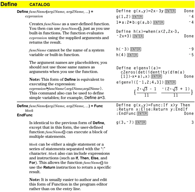
Creates funcName as a user-defined function. You then can use funcName(), just as you use built-in functions. The function evaluates expression using the supplied arguments and returns the result.
funcName cannot be the name of a system variable or built-in function.
The argument names are placeholders; you should not use those same names as arguments when you use the function.
Note: This form of Define is equivalent to executing the expression: expression►funcName( arg1Name, arg2Name). This command also can be used to define simple variables; for example, Define a=3.
Define g(x,y)=2x-3y [ENTER] Done g(1,2) [ENTER] -4 1⇒a:2⇒b:g(a,b) [ENTER] -4
Define h(x)=when(x<2,2x-3, -2x+3) [ENTER] Done h(-3) [ENTER] -9 h(4) [ENTER] -5
Define eigenvl(a)= cZeros(det(identity(dim(a) [1])-x*a),x) [ENTER] Done eigenvl([-1,2;4,3]) [ENTER] { (2√3 - 1)/11 -(2√3 + 1)/11 }
Define funcName(arg1Name, arg2Name, ...) = Func block EndFunc
Is identical to the previous form of Define, except that in this form, the user-defined function funcName() can execute a block of multiple statements.
block can be either a single statement or a series of statements separated with the “;” character. block also can include expressions and instructions (such as If, Then, Else, and For). This allows the function funcName() to use the Return instruction to return a specific result.
Note: It is usually easier to author and edit this form of Function in the program editor rather than on the entry line.
Define g(x,y)=Func:If x>y Then :Return x:Else:Return y:EndIf :EndFunc [ENTER] Done g(3,-7) [ENTER] 3
Appendix A: Functions and Instructions 433
Define progName(arg1Name, arg2Name, ...) = Prgm block EndPrgm
Creates progName as a program or subprogram, but cannot return a result using Return. Can execute a block of multiple statements.
block can be either a single statement or a series of statements separated with the “:” character. block also can include expressions and instructions (such as If, Then, Else, and For) without restrictions.
Note: It is usually easier to author and edit a program block in the Program Editor rather than on the entry line.
Define listinpt()=prgm:Local n,i,str1,num:InputStr "Enter name of list",str1:Input "No. of elements",n:For i,1,n,1:Input "element "&string(i),num: num⇒str1[i]:EndFor:EndPrgm [ENTER] Done listinpt() [ENTER] Enter name of list
DelFold CATALOG
DelFold folderName1[, folderName2][, folderName3] ...
Deletes user-defined folders with the names folderName1, folderName2, etc. An error message is displayed if the folders contain any variables.
Note: You cannot delete the main folder.
NewFold games [ENTER] Done (creates the folder games) DelFold games [ENTER] Done (deletes the folder games)
DelVar CATALOG
DelVar var1[, var2][, var3] ...
Deletes the specified variables from memory.
2⇒a [ENTER] 2 (a+2)^2 [ENTER] 16 DelVar a [ENTER] Done (a+2)^2 [ENTER] (a + 2)²
deSolve() MATH/Calculus menu
deSolve(1stOr2ndOrderOde, independentVar, dependentVar) ⇒ a general solution
Returns an equation that explicitly or implicitly specifies a general solution to the 1st- or 2nd-order ordinary differential equation (ODE). In the ODE:
• Use a prime symbol (' , press [2nd] [·]) to denote the 1st derivative of the dependent variable with respect to the independent variable.
• Use two prime symbols to denote the corresponding second derivative.
The ' symbol is used for derivatives within deSolve() only. In other cases, use d().
The general solution of a 1st-order equation contains an arbitrary constant of the form @k, where k is an integer suffix from 1 through 255. The suffix resets to 1 when you use ClrHome or [F8]: Clear Home. The solution of a 2nd-order equation contains two such constants.
Note: To type a prime symbol ('), press [2nd] [·].
deSolve(y''+y'+y=x^2,x,y) [ENTER] y=(@1·x+@2)·e^(-x)+x^2 - 4·x+6 right(ans(1))⇒temp [ENTER] (@1·x+@2)·e^(-x)+x^2 - 4·x+6 d(temp,x,2)+2*d(temp,x)+temp-x^2 [ENTER] 0 DelVar temp [ENTER] Done
434 Appendix A: Functions and Instructions
Apply solve() to an implicit solution if you want to try to convert it to one or more equivalent explicit solutions.
When comparing your results with textbook or manual solutions, be aware that different methods introduce arbitrary constants at different points in the calculation, which may produce different general solutions.
deSolve(1stOrderOde and initialCondition, independentVar, dependentVar) ⇒ a particular solution
Returns a particular solution that satisfies 1stOrderOde and initialCondition. This is usually easier than determining a general solution, substituting initial values, solving for the arbitrary constant, and then substituting that value into the general solution.
initialCondition is an equation of the form:
dependentVar (initialIndependentValue) = initialDependentValue
The initialIndependentValue and initialDependentValue can be variables such as x0 and y0 that have no stored values. Implicit differentiation can help verify implicit solutions.
deSolve(2ndOrderOde and initialCondition1 and initialCondition2, independentVar, dependentVar) ⇒ a particular solution
Returns a particular solution that satisfies 2ndOrderOde and has a specified value of the dependent variable and its first derivative at one point.
For initialCondition1, use the form:
dependentVar (initialIndependentValue) = initialDependentValue
For initialCondition2, use the form:
dependentVar' (initialIndependentValue) = initial1stDerivativeValue
\begin{tabular}{p{0.55\textwidth} p{0.4\textwidth}} & deSolve(y'=(cos(y))^2x,x,y) \ & \text{ENTER} \ & \tan(y)=x^2/2 +@3 \ & solve(ans(1),y) \text{ENTER} \ & y=\tan^-1\left(x^2+2\cdot@3/2\right) +n1\cdot\pi \ & \textbf{Note:} To type an @ symbol, press: \ & TI-89: \textbullet{} STO\blacktriangleright \ & TI-92 Plus: 2nd R \ & ans(1) |@3=c-1 and @n1=0 \text{ENTER} \ & y=\tan^-1\left(x^2+2\cdot(c-1)/2\right) \ & sin(y)=(ye^(x)+cos(y))y'→ode \ & \text{ENTER} \ & \sin(y)=(e^x\cdot y+\cos(y))\cdot y' \ & deSolve(ode and y(0)=0,x,y)→soln \text{ENTER} \ & -(2\cdot\sin(y)+y^2)/2=-(e^x-1)\cdot e^x\cdot\sin(y) \ & soln|x=0 and y=0 \text{ENTER} \quad true \ & d(right(eq)-left(eq),x)/ \ & (d(left(eq)-right(eq),y)) \ & →impdif(eq,x,y) \text{ENTER} \ & \quad Done \ & ode|y'=impdif(soln,x,y) \text{ENTER} \ & \quad true \ & DelVar ode,soln \text{ENTER} \quad Done \ & deSolve(y''=y^(-1/2) and y(0)=0 and y'(0)=0,t,y) \text{ENTER} \ & \frac2\cdot y^3/43=t \ & solve(ans(1),y) \text{ENTER} \ & y=\frac2^2/3\cdot(3\cdot t)^4/34 and t\geq0 \ \end{tabular}
Appendix A: Functions and Instructions 435
deSolve(2ndOrderOde and boundaryCondition1 and boundaryCondition2, independentVar, dependentVar) \Rightarrow a particular solution
Returns a particular solution that satisfies 2ndOrderOde and has specified values at two different points.
deSolve(w''-2w'/x+(9+2/x^2)w= x*e^(x) and w(\pi/6)=0 and w(\pi/3)=0,x,w) [ENTER]
$$ w=\frac{e^{\frac{\pi}{3}} \cdot x \cdot \cos(3 \cdot x)}{10} - \frac{e^{\frac{\pi}{6}} \cdot x \cdot \sin(3 \cdot x)}{10} + \frac{x \cdot e^x}{10} $$
det() MATH/Matrix menu
det(squareMatrix[, tol]) \Rightarrow expression
Returns the determinant of squareMatrix.
Optionally, any matrix element is treated as zero if its absolute value is less than tol. This tolerance is used only if the matrix has floating-point entries and does not contain any symbolic variables that have not been assigned a value. Otherwise, tol is ignored.
- If you use [\blacklozenge][ENTER] or set the mode to Exact/Approx=APPROXIMATE, computations are done using floating-point arithmetic.
- If tol is omitted or not used, the default tolerance is calculated as:
5\varepsilon^-14 * max(dim(squareMatrix))
- rowNorm(squareMatrix)
det([a,b;c,d]) [ENTER] a \cdot d - b \cdot c
det([1,2;3,4]) [ENTER] -2
det(identity(3)-x*[1,-2,3; -2,4,1;-6,-2,7]) [ENTER] -(98 \cdot x$^3$ - 55 \cdot x$^2$ + 12 \cdot x - 1)
[1E20,1;0,1] \rightarrowmat1 det(mat1) [ENTER] det(mat1,1) [ENTER]
$$ \begin{bmatrix} 1.\varepsilon20 & 1 \ 0 & 1 \end{bmatrix} $$ 0 1.\varepsilon20
diag() MATH/Matrix menu
diag(list) \Rightarrow matrix diag(rowMatrix) \Rightarrow matrix diag(columnMatrix) \Rightarrow matrix
Returns a matrix with the values in the argument list or matrix in its main diagonal.
diag({2,4,6}) [ENTER]
$$ \begin{bmatrix} 2 & 0 & 0 \ 0 & 4 & 0 \ 0 & 0 & 6 \end{bmatrix} $$
diag(squareMatrix) \Rightarrow rowMatrix
Returns a row matrix containing the elements from the main diagonal of squareMatrix.
squareMatrix must be square.
[4,6,8;1,2,3;5,7,9] [ENTER]
$$ \begin{bmatrix} 4 & 6 & 8 \ 1 & 2 & 3 \ 5 & 7 & 9 \end{bmatrix} $$
diag(ans(1)) [ENTER] [4 2 9]
436 Appendix A: Functions and Instructions
Dialog CATALOG
Dialog block EndDlg
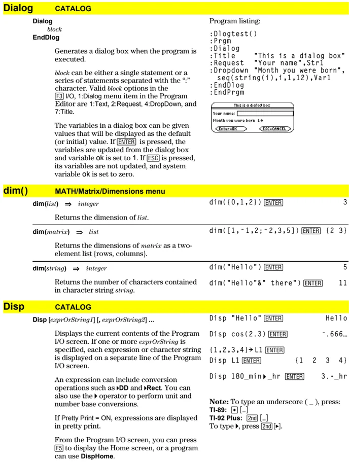
Generates a dialog box when the program is executed.
block can be either a single statement or a series of statements separated with the “:” character. Valid block options in the [F3] I/O, 1:Dialog menu item in the Program Editor are 1:Text, 2:Request, 4:DropDown, and 7:Title.
The variables in a dialog box can be given values that will be displayed as the default (or initial) value. If [ENTER] is pressed, the variables are updated from the dialog box and variable ok is set to 1. If [ESC] is pressed, its variables are not updated, and system variable ok is set to zero.
Program listing: :Dlogtest() :Prgm :Dlg :Title "This is a dialog box" :Request "Your name",Str1 :DropDown "Month you were born", seq(string(i),i,1,12),Var1 :EndDlg :EndPrgm
dim() MATH/Matrix/Dimensions menu
dim(list) \Rightarrow integer Returns the dimension of list. dim({0,1,2}) [ENTER] 3
dim(matrix) \Rightarrow list Returns the dimensions of matrix as a two-element list {rows, columns}. dim([1,-1,2;-2,3,5]) [ENTER] {2 3}
dim(string) \Rightarrow integer Returns the number of characters contained in character string string. dim("Hello") [ENTER] 5 dim("Hello"&" there") [ENTER] 11
Disp CATALOG
Disp [exprOrString1] [, exprOrString2] ... Displays the current contents of the Program I/O screen. If one or more exprOrString is specified, each expression or character string is displayed on a separate line of the Program I/O screen.
An expression can include conversion operations such as \blacktrianglerightDD and \blacktrianglerightRect. You can also use the \blacktriangleright operator to perform unit and number base conversions.
If Pretty Print = ON, expressions are displayed in pretty print.
From the Program I/O screen, you can press [F5] to display the Home screen, or a program can use DispHome.
Disp "Hello" [ENTER] Hello Disp cos(2.3) [ENTER] -.666... {1,2,3,4}\blacktrianglerightL1 [ENTER] Disp L1 [ENTER] {1 2 3 4} Disp 180_min\blacktriangleright_hr [ENTER] 3.\cdot _hr
Note: To type an underscore (), press: TI-89: [\blacklozenge] [] TI-92 Plus: [2nd] [_] To type \blacktriangleright, press [2nd] [\blacktriangleright].
Appendix A: Functions and Instructions 437
DispG CATALOG
DispG Displays the current contents of the Graph screen.
In function graphing mode:
Program segment: \vdots :5*\cos(x)\rightarrow y1(x) :-10\rightarrow xmin :10\rightarrow xmax :-5\rightarrow ymin :5\rightarrow ymax $:DispG$ \vdots
DispHome CATALOG
DispHome Displays the current contents of the Home screen.
Program segment: \vdots $:Disp "The result is: ",xx$ $:Pause "Press Enter to quit"$ $:DispHome$ $:EndPrgm$
DispTbl CATALOG
DispTbl Displays the current contents of the Table screen.
Note: The cursor pad is active for scrolling. Press \boxedESC or \boxedENTER to resume execution if in a program.
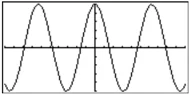
5*\cos(x)\rightarrow y1(x) \boxedENTER $DispTbl$ \boxedENTER
\blacktrianglerightDMS MATH/Angle menu
expression \blacktrianglerightDMS list \blacktrianglerightDMS matrix \blacktrianglerightDMS
Interprets the argument as an angle and displays the equivalent DMS (DDDDDD° MM' SS.ss'') number. See °, ', '' on page 536 for DMS (degree, minutes, seconds) format.
Note: \blacktrianglerightDMS will convert from radians to degrees when used in radian mode. If the input is followed by a degree symbol (°), no conversion will occur. You can use \blacktrianglerightDMS only at the end of an entry line.
In Degree angle mode: 45.371 \blacktrianglerightDMS \boxedENTER 45° 22' 15.6''
\45.371,60\ \blacktrianglerightDMS \boxedENTER \45° 22' 15.6'' \quad 60° \
438 Appendix A: Functions and Instructions
dotP() MATH/Matrix/Vector ops menu
dotP(list1, list2) \Rightarrow expression Returns the “dot” product of two lists.
dotP({a,b,c},{d,e,f}) ENTER a \cdot d + b \cdot e + c \cdot f
dotP({1,2},{5,6}) ENTER 17
dotP(vector1, vector2) \Rightarrow expression Returns the “dot” product of two vectors. Both must be row vectors, or both must be column vectors.
dotP([a,b,c],[d,e,f]) ENTER a \cdot d + b \cdot e + c \cdot f
dotP([1,2,3],[4,5,6]) ENTER 32
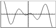
DrawFunc CATALOG
DrawFunc expression Draws expression as a function, using x as the independent variable. Note: Regraphing erases all drawn items.
In function graphing mode and ZoomStd window: DrawFunc 1.25x*cos(x) ENTER
DrawInv CATALOG
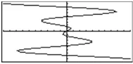
DrawInv expression Draws the inverse of expression by plotting x values on the y axis and y values on the x axis. x is the independent variable. Note: Regraphing erases all drawn items.
In function graphing mode and ZoomStd window: DrawInv 1.25x*cos(x) ENTER
DrawParm CATALOG
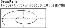
DrawParm expression1, expression2 [, tmin] [, tmax] [, tstep] Draws the parametric equations expression1 and expression2, using t as the independent variable. Defaults for tmin, tmax, and tstep are the current settings for the Window variables tmin, tmax, and tstep. Specifying values does not alter the window settings. If the current graphing mode is not parametric, these three arguments are required. Note: Regraphing erases all drawn items.
In function graphing mode and ZoomStd window: DrawParm tcos(t),tsin(t),0,10,.1 ENTER
Appendix A: Functions and Instructions 439
DrawPol CATALOG
DrawPol expression[, \thetamin] [, \thetamax] [, \thetastep]
Draws the polar graph of expression, using \theta as the independent variable.
Defaults for \thetamin, \thetamax, and \thetastep are the current settings for the Window variables \thetamin, \thetamax, and \thetastep. Specifying values does not alter the window settings. If the current graphing mode is not polar, these three arguments are required.
Note: Regraphing erases all drawn items.
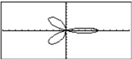
In function graphing mode and ZoomStd window:
DrawPol 5*cos(3\theta),0,3.5,.1
[ENTER]
DrawSlp CATALOG
DrawSlp x1, y1, slope
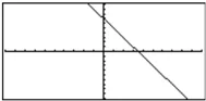
Displays the graph and draws a line using the formula y - y1 = slope \cdot (x - x1).
Note: Regraphing erases all drawn items.
In function graphing mode and ZoomStd window:
DrawSlp 2,3,-2 [ENTER]
DropDown CATALOG
DropDown titleString, {item1String, item2String, ...}, varName
Displays a drop-down menu with the name titleString and containing the items 1:item1String, 2:item2String, and so forth. DropDown must be within a Dialog...EndDlog block.
If varName already exists and has a value within the range of items, the referenced item is displayed as the default selection. Otherwise, the menu's first item is the default selection.
When you select an item from the menu, the corresponding number of the item is stored in the variable varName. (If necessary, DropDown creates varName.)
See Dialog program listing example.
440 Appendix A: Functions and Instructions
DrwCtour CATALOG
DrwCtour expression
DrwCtour list
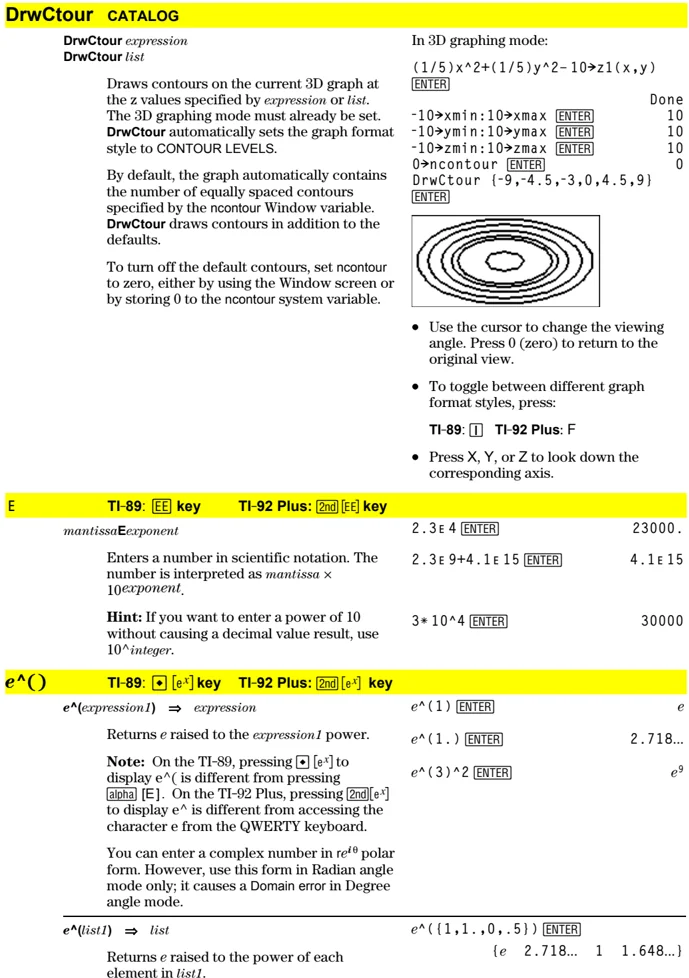
Draws contours on the current 3D graph at the z values specified by expression or list. The 3D graphing mode must already be set. DrwCtour automatically sets the graph format style to CONTOUR LEVELS.
By default, the graph automatically contains the number of equally spaced contours specified by the ncontour Window variable. DrwCtour draws contours in addition to the defaults.
To turn off the default contours, set ncontour to zero, either by using the Window screen or by storing 0 to the ncontour system variable.
In 3D graphing mode:
(1/5)x^2+(1/5)y^2-10→z1(x,y) ENTER
-10→xmin:10→xmax ENTER Done -10→ymin:10→ymax ENTER 10 -10→zmin:10→zmax ENTER 10 0→ncontour ENTER 0 DrwCtour {-9,-4.5,-3,0,4.5,9} ENTER
- Use the cursor to change the viewing angle. Press 0 (zero) to return to the original view.
- To toggle between different graph format styles, press:
- TI-89: [I] TI-92 Plus: F
- Press X, Y, or Z to look down the corresponding axis.
E
TI-89: [EE] key
TI-92 Plus: [2nd] [EE] key
mantissaEexponent
Enters a number in scientific notation. The number is interpreted as mantissa × 10^exponent.
Hint: If you want to enter a power of 10 without causing a decimal value result, use 10^integer.
2.3E4 ENTER 23000. 2.3E9+4.1E15 ENTER 4.1E15 3*10^4 ENTER 30000
e^()
TI-89: [♦] [e^x] key
TI-92 Plus: [2nd] [e^x] key
e^(expression1) ⇒ expression
Returns e raised to the expression1 power.
Note: On the TI-89, pressing [♦] [e^x] to display e^( is different from pressing [alpha] [E]. On the TI-92 Plus, pressing [2nd][e^x] to display e^ is different from accessing the character e from the QWERTY keyboard.
You can enter a complex number in re^(iθ) polar form. However, use this form in Radian angle mode only; it causes a Domain error in Degree angle mode.
e^(1) ENTER e e^(1.) ENTER 2.718... e^(3)^2 ENTER e^9
e^(list1) ⇒ list
Returns e raised to the power of each element in list1.
e^({1,1.,0,.5}) ENTER {e 2.718... 1 1.648...}
Appendix A: Functions and Instructions 441
e^(squareMatrix1) \Rightarrow squareMatrix
Returns the matrix exponential of squareMatrix1. This is not the same as calculating $e$ raised to the power of each element. For information about the calculation method, refer to cos().
squareMatrix1 must be diagonalizable. The result always contains floating-point numbers.
e^([1,5,3;4,2,1;6,-2,1]) ENTER
$$ \begin{bmatrix} 782.209 & 559.617 & 456.509 \ 680.546 & 488.795 & 396.521 \ 524.929 & 371.222 & 307.879 \end{bmatrix} $$
eigVc() MATH/Matrix menu
eigVc(squareMatrix) ⇒ matrix
Returns a matrix containing the eigenvectors for a real or complex squareMatrix, where each column in the result corresponds to an eigenvalue. Note that an eigenvector is not unique; it may be scaled by any constant factor. The eigenvectors are normalized, meaning that if V = [x_1, x_2, \ldots, x_n], then:
$$ \sqrt{x_1^2 + x_2^2 + \ldots + x_n^2} = 1 $$
squareMatrix is first balanced with similarity transformations until the row and column norms are as close to the same value as possible. The squareMatrix is then reduced to upper Hessenberg form and the eigenvectors are computed via a Schur factorization.
In Rectangular complex format mode:
[-1,2,5;3,-6,9;2,-5,7] → m1 ENTER
$$ \begin{bmatrix} -1 & 2 & 5 \ 3 & -6 & 9 \ 2 & -5 & 7 \end{bmatrix} $$
eigVc(m1) ENTER
$$ \begin{bmatrix} -.800... & .767... & .767... \
- 484... & .573...+.052...·i & .573...-.052...·i \
- 352... & .262...+.096...·i & .262...-.096...·i \end{bmatrix} $$
eigVl() MATH/Matrix menu
eigVl(squareMatrix) ⇒ list
Returns a list of the eigenvalues of a real or complex squareMatrix.
squareMatrix is first balanced with similarity transformations until the row and column norms are as close to the same value as possible. The squareMatrix is then reduced to upper Hessenberg form and the eigenvalues are computed from the upper Hessenberg matrix.
In Rectangular complex format mode:
[-1,2,5;3,-6,9;2,-5,7] → m1 ENTER
$$ \begin{bmatrix} -1 & 2 & 5 \ 3 & -6 & 9 \ 2 & -5 & 7 \end{bmatrix} $$
eigVl(m1) ENTER
$$ {-4.409... \quad 2.204...+.763...·i \quad 2.204...-.763...·i} $$
Else
See If, page 456.
Elself
CATALOG See also If, page 456.
If Boolean expression1 Then
block1
Elself Boolean expression2 Then
block2
:
Elself Boolean expressionN Then
blockN
EndIf
:
Elself can be used as a program instruction for program branching.
Program segment:
: :If choice=1 Then : Goto option1 : Elself choice=2 Then : Goto option2 : Elself choice=3 Then : Goto option3 : Elself choice=4 Then : Disp "Exiting Program" : Return :EndIf :
442 Appendix A: Functions and Instructions
EndCustm See Custom, page 429.
EndDlog See Dialog, page 437.
EndFor See For, page 450.
EndFunc See Func, page 451.
EndIf See If, page 456.
EndLoop See Loop, page 466.
EndPrgm See Prgm, page 481.
EndTBar See ToolBar, page 515.
EndTry See Try, page 515.
EndWhile See While, page 518.
entry() CATALOG
entry() \Rightarrow expression entry(integer) \Rightarrow expression
Returns a previous entry-line entry from the Home screen history area.
integer, if included, specifies which entry expression in the history area. The default is 1, the most recently evaluated entry. Valid range is from 1 to 99 and cannot be an expression.
Note: If the last entry is still highlighted on the Home screen, pressing [ENTER] is equivalent to executing entry(1).
On the Home screen:
1+1/x [ENTER] 1/x + 1
1+1/entry(1) [ENTER] 2 - 1/x+1
[ENTER] 1/2 \cdot (2 \cdot x+1) + 3/2
[ENTER] 5/3 - 1/3 \cdot (3 \cdot x+2)
entry(4) [ENTER] 1/x + 1
exact() MATH/Number menu
exact(expression1 [, tol]) \Rightarrow expression exact(list1 [, tol]) \Rightarrow list exact(matrix1 [, tol]) \Rightarrow matrix
Uses Exact mode arithmetic regardless of the Exact/Approx mode setting to return, when possible, the rational-number equivalent of the argument.
tol specifies the tolerance for the conversion; the default is 0 (zero).
exact(.25) [ENTER] 1/4
exact(.333333) [ENTER] 333333/1000000
exact(.33333,.001) 1/3
exact(3.5x+y) [ENTER] 7 \cdot x/2 + y
exact({.2,.33,4.125}) [ENTER] {1/5 33/100 33/8}
Appendix A: Functions and Instructions 443
Exec CATALOG
Exec string [, expression1] [, expression2] ...
Executes a string consisting of a series of Motorola 68000 op-codes. These codes act as a form of an assembly-language program. If needed, the optional expressions let you pass one or more arguments to the program.
For more information, check the TI Web site: education.ti.com
Warning: Exec gives you access to the full power of the microprocessor. Please be aware that you can easily make a mistake that locks up the calculator and causes you to lose your data. We suggest you make a backup of the calculator contents before attempting to use the Exec command.
Exit CATALOG
Exit
Exits the current For, While, or Loop block.
Exit is not allowed outside the three looping structures (For, While, or Loop).
Program listing: :0\rightarrowtemp :For i,1,100,1 : temp+i\rightarrowtemp : If temp>20 : Exit :EndFor :Disp temp
Contents of temp after execution: 21
exp\blacktrianglerightlist() CATALOG
exp\blacktrianglerightlist(expression,var) \Rightarrow list
Examines expression for equations that are separated by the word "or," and returns a list containing the right-hand sides of the equations of the form var=expression. This gives you an easy way to extract some solution values embedded in the results of the solve(), cSolve(), fMin(), and fMax() functions.
Note: exp\blacktrianglerightlist() is not necessary with the zeros and cZeros() functions because they return a list of solution values directly.
solve(x^2-x-2=0,x) [ENTER] x=2 or x=-1
exp\blacktrianglerightlist(solve(x^2-x-2=0,x),x) [ENTER] {-1 2}
444 Appendix A: Functions and Instructions
expand() MATH/Algebra menu
expand(expression1 [, var]) \Rightarrow expression expand(list1 [,var]) \Rightarrow list expand(matrix1 [var]) \Rightarrow matrix
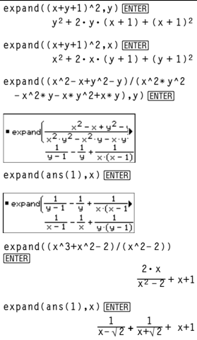
expand(expression1) returns expression1 expanded with respect to all its variables. The expansion is polynomial expansion for polynomials and partial fraction expansion for rational expressions.
The goal of expand() is to transform expression1 into a sum and/or difference of simple terms. In contrast, the goal of factor() is to transform expression1 into a product and/or quotient of simple factors.
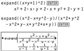
\begin{tabular}{p{0.5\textwidth} p{0.45\textwidth}} expand((x+y+1)^2) \textbf{ENTER} & \ & x^2 + 2 \cdot x \cdot y + 2 \cdot x + y^2 + 2 \cdot y + 1 \ expand((x^2-x+y^2-y)/(x^2*y^2 & \
- x^2y - xy^2+xy)) \textbf{ENTER} & \ \blacksquare expand \left( x^2 - x + y^2 - y/x^2 \cdot y^2 - x^2 \cdot y - x \cdot y^2 + x \cdot y \right) & \ = 1/x-1 - 1/x + 1/y-1 - 1/y & \ \hline expand(expression1,var) returns expression expanded with respect to var. Similar powers of var are collected. The terms and their factors are sorted with var as the main variable. There might be some incidental factoring or expansion of the collected coefficients. Compared to omitting var, this often saves time, memory, and screen space, while making the expression more comprehensible. & expand((x+y+1)^2,y) \textbf{ENTER} \ & y^2 + 2 \cdot y \cdot (x + 1) + (x + 1)^2 \ expand((x+y+1)^2,x) \textbf{ENTER} & \ & x^2 + 2 \cdot x \cdot (y + 1) + (y + 1)^2 \ expand((x^2-x+y^2-y)/(x^2y^2 & \
- x^2y - xy^2+x*y),y) \textbf{ENTER} & \ \blacksquare expand \left( x^2 - x + y^2 - y/x^2 \cdot y^2 - x^2 \cdot y - x \cdot y^2 + x \cdot y \right) & \ = 1/y-1 - 1/y + 1/x \cdot (x-1) & \ expand(ans(1),x) \textbf{ENTER} & \ \blacksquare expand \left( 1/y-1 - 1/y + 1/x \cdot (x-1) \right) & \ = 1/x-1 - 1/x + 1/y \cdot (y-1) & \ Even when there is only one variable, using var might make the denominator factorization used for partial fraction expansion more complete. & expand((x^3+x^2-2)/(x^2-2)) \textbf{ENTER} \ & 2 \cdot x/x^2 - 2 + x + 1 \ \textbf{Hint:} For rational expressions, propFrac() is a faster but less extreme alternative to expand(). & expand(ans(1),x) \textbf{ENTER} \ & \frac1x-\sqrt2 + \frac1x+\sqrt2 + x+1 \ \textbf{Note:} See also comDenom() for an expanded numerator over an expanded denominator. & \ \end{tabular}
Appendix A: Functions and Instructions 445
expand(expression1,[var]) also distributes logarithms and fractional powers regardless of var. For increased distribution of logarithms and fractional powers, inequality constraints might be necessary to guarantee that some factors are nonnegative.
expand(expression1, [var]) also distributes absolute values, sign(), and exponentials, regardless of var.
Note: See also tExpand() for trigonometric angle-sum and multiple-angle expansion.
expr() MATH/String menu
expr(string) \Rightarrow expression
Returns the character string contained in string as an expression and immediately executes it.
expr("1+2+x^2+x") ENTER $x^2 + x + 3$ expr("expand((1+x)^2)") ENTER x^2 + 2 \cdot x + 1 "Define cube(x)=x^3">funcstr ENTER "Define cube(x)=x^3" expr(funcstr) ENTER Done cube(2) ENTER 8
ExpReg MATH/Statistics/Regressions menu
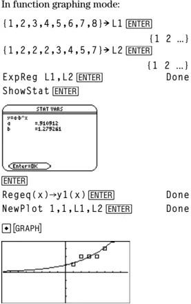
ExpReg list1, list2 [, [list3] [, list4, list5]]
Calculates the exponential regression and updates all the system statistics variables. All the lists must have equal dimensions except for list5. list1 represents xlist. list2 represents ylist. list3 represents frequency. list4 represents category codes. list5 represents category include list.
Note: list1 through list4 must be a variable name or c1–c99 (columns in the last data variable shown in the Data/Matrix Editor). list5 does not have to be a variable name and cannot be c1–c99.
In function graphing mode:
{1,2,3,4,5,6,7,8}→L1 ENTER {1 2 ...} {1,2,2,2,3,4,5,7}→L2 ENTER {1 2 ...} ExpReg L1,L2 ENTER Done ShowStat ENTER
ENTER Regeq(x)→y1(x) ENTER Done NewPlot 1,1,L1,L2 ENTER Done
446 Appendix A: Functions and Instructions
factor() MATH/Algebra menu
factor(expression1[, var]) ⇒ expression
factor(list1[,var]) ⇒ list
factor(matrix1[,var]) ⇒ matrix
factor(expression1) returns expression1 factored with respect to all of its variables over a common denominator.
expression1 is factored as much as possible toward linear rational factors without introducing new non-real subexpressions. This alternative is appropriate if you want factorization with respect to more than one variable.
factor(expression1,var) returns expression1 factored with respect to variable var.
expression1 is factored as much as possible toward real factors that are linear in var, even if it introduces irrational constants or subexpressions that are irrational in other variables.
The factors and their terms are sorted with var as the main variable. Similar powers of var are collected in each factor. Include var if factorization is needed with respect to only that variable and you are willing to accept irrational expressions in any other variables to increase factorization with respect to var. There might be some incidental factoring with respect to other variables.
For the AUTO setting of the Exact/Approx mode, including var permits approximation with floating-point coefficients where irrational coefficients cannot be explicitly expressed concisely in terms of the built-in functions. Even when there is only one variable, including var might yield more complete factorization.
Note: See also comDenom() for a fast way to achieve partial factoring when factor() is not fast enough or if it exhausts memory.
Note: See also cFactor() for factoring all the way to complex coefficients in pursuit of linear factors.
factor(a^3x^2 - ax^2 - a^3 + a)
ENTER
a·(a - 1)·(a + 1)·(x - 1)·(x + 1)
factor(x^2 + 1) ENTER
x² + 1
factor(x^2 - 4) ENTER
(x - 2)·(x + 2)
factor(x^2 - 3) ENTER
x² - 3
factor(x^2 - a) ENTER
x² - a
factor(a^3x^2 - ax^2 - a^3 + a, x)
ENTER
a·(a² - 1)·(x - 1)·(x + 1)
factor(x^2 - 3, x) ENTER
(x + √3)·(x - √3)
factor(x^2 - a, x) ENTER
(x + √a)·(x - √a)
factor(x^5 + 4x^4 + 5x^3 - 6x - 3)
ENTER
x⁵ + 4·x⁴ + 5·x³ - 6·x - 3
factor(ans(1), x) ENTER
(x - .964...)·(x + .611...)·
(x + 2.125...)·(x² + 2.227...·x + 2.392...)
Appendix A: Functions and Instructions 447
factor(rationalNumber) returns the rational number factored into primes. For composite numbers, the computing time grows exponentially with the number of digits in the second-largest factor. For example, factoring a 30-digit integer could take more than a day, and factoring a 100-digit number could take more than a century.
Note: To stop (break) a computation, press [ON].
If you merely want to determine if a number is prime, use isPrime() instead. It is much faster, particularly if rationalNumber is not prime and if the second-largest factor has more than five digits.
\begin{tabular}{p{0.45\textwidth} p{0.45\textwidth}} \textbf{Fill} \quad MATH/Matrix menu & \ Fill expression, matrixVar \Rightarrow matrix & factor(152417172689) \texttt{ENTER} \ Replaces each element in variable matrixVar with expression. & 123457\cdot1234577 \ matrixVar must already exist. & isPrime(152417172689) \texttt{ENTER}false \ & [1,2;3,4]\blacktrianglerightamatrx \texttt{ENTER} \
- & \quad \quad \quad \quad \quad \quad \quad \quad \quad \quad \quad \quad \quad \quad \quad \quad \quad \quad \quad \quad \quad \quad \quad \quad \quad \quad \quad \quad \quad \quad \quad \quad \quad \quad \quad \quad \quad \quad \quad \quad \quad \quad \quad \quad \ ........ \begin{tabular}{@{}cc@{}}1 & 2 \ 3 & 4\end{tabular} \ & Fill 1.01,amatrx \texttt{ENTER} \
- & \quad \quad \quad \quad \quad \quad \quad \quad \quad \quad \quad \quad \quad \quad \quad \quad \quad \quad \quad \quad \quad \quad \quad \quad \quad \quad \quad \quad \quad \quad \quad \quad \quad \quad \quad \quad \quad \quad \quad \quad \quad \quad \quad \quad \quad \quad \quad \quad \quad \quad \quad \quad \quad \quad \quad \quad \quad \quad \quad \quad \quad \quad \quad \quad \quad \quad ........ Done \ & amatrx \texttt{ENTER} \
- & \quad \quad \quad \quad \quad \quad \quad \quad \quad \quad \quad \quad \quad \quad \quad \quad \quad \quad \quad \quad \quad \quad \quad \quad \quad \quad \quad \quad \quad \quad \quad \quad \quad \quad ........
Use the “|” operator to restrict the solution interval and/or specify the sign of other undefined variables.
For the APPROX setting of the Exact/Approx mode, fMax() iteratively searches for one approximate local maximum. This is often faster, particularly if you use the “|” operator to constrain the search to a relatively small interval that contains exactly one local maximum.
Note: See also fMin() and max().
fMax(.5x^3-x-2,x)|x≤1 [ENTER] x = -.816...
fMax(a*x^2,x) [ENTER] x = ∞ or x = -∞ or x = 0 or a = 0
fMax(a*x^2,x)|a<0 [ENTER] x = 0
fMin() MATH/Calculus menu
fMin(expression, var) \Rightarrow Boolean expression
Returns a Boolean expression specifying candidate values of var that minimize expression or locate its greatest lower bound.
Use the “|” operator to restrict the solution interval and/or specify the sign of other undefined variables.
For the APPROX setting of the Exact/Approx mode, fMin() iteratively searches for one approximate local minimum. This is often faster, particularly if you use the “|” operator to constrain the search to a relatively small interval that contains exactly one local minimum.
Note: See also fMax() and min().
fMin(1-(x-a)^2-(x-b)^2,x) [ENTER] x = ∞ or x = -∞
fMin(.5x^3-x-2,x)|x≥1 [ENTER] x = 1
fMin(a*x^2,x) [ENTER] x = ∞ or x = -∞ or x = 0 or a = 0
fMin(a*x^2,x)|a>0 and x>1 [ENTER] x = 1.
fMin(a*x^2,x)|a>0 [ENTER] x = 0
FnOff CATALOG
FnOff
Deselects all Y= functions for the current graphing mode.
In split-screen, two-graph mode, FnOff only applies to the active graph.
FnOff [1] [, 2] ... [,99]
Deselects the specified Y= functions for the current graphing mode.
In function graphing mode: FnOff 1,3 [ENTER] deselects y1(x) and y3(x).
In parametric graphing mode: FnOff 1,3 [ENTER] deselects xt1(t), yt1(t), xt3(t), and yt3(t).
FnOn CATALOG
FnOn
Selects all Y= functions that are defined for the current graphing mode.
In split-screen, two-graph mode, FnOn only applies to the active graph.
Appendix A: Functions and Instructions 449